Self-Similarity and Fractal Structure

There is not just one timeline in the brain, there are many. We can arbitrarily construct such a timeline at any level of resolution, not just for the neural network as a whole but also for the neurons and synapses (even molecules) within it. What is the significance of a collection of time series relative to internal events? The importance of the time element becomes immediately obvious when we begin to consider Markov and non-Markov behavior in neural networks. But before getting into that, we can consider what happens when the extent of the mapping interval varies.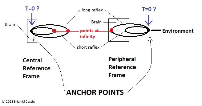

Some reflexes are fast, others are slow. Some pathways are myelinated, others aren't. Gap junctions are a bit faster than chemical synapses. And molecular kinetics are important for both regulation and engagement in individual synapses. How do we put all this together?

The figure defines a concept called "anchor", which we'll use in various ways during this discussion. Loosely speaking, it's related to where we put the electrode, which in turn defines our mapping origin T=0. From the standpoint of a black box (the organism) interacting with the environment, we can arbitarily define the origin to be the environmental interface, because we can easily measure it (at least, more easily than invading the black box in most cases). And, this definition also makes sense from the point of view of a central timeline, because the origin is then by definition the point of singularity.

One convenient way to visualize relationships between brain activities is graphically, geometrically. Things sometimes become clearer this way. For example the brain devotes over half its neurons to processing a small region of the timeline. There is a specific reason for this, given the brain's architecture, and once we understand it, the reason for other things becomes clear too. The point in question though, is not what one might think at first - it's not the singularity around T=0 (even though that's what it's modeling). Compactness means to make compact. It means there's no holes in our timeline. However, we've already identified one. And worse, the required real-time optimization occurs exactly at the point of singularity! So how do we cover this hole? Is there perhaps more than one hole, that we need to cover?

As noted on the previous page, compactification creates a "point at infinity" through which signals can travel. If we were looking at the same thing on the original linear timeline, information would seem to drop off the left (sensory) end and reappear on the right (motor) end. But in the compactified timeline, it simply continues traveling around the circle, maintaining the same orientation while it does. Compactification creates a loop topology, which becomes even more interesting when it's applied globally.

The Hawaiian Earring

Considering brain architecture in terms of feedback loops, it is clear that there are many loops with differing conduction delays. A monosynaptic reflex arc through the neck will have a shorter loop time than one through the toe. A molecular loop could be on the order of microseconds, while a circadian loop takes days. The various loop times result in differing radii after we compactify the associated timelines. In a very large network consisting of billions of neurons, we can imagine a rich loop structure, in such a way that for any given radius, we are likely to find an example of it - or at least an example near it. In other words, the loops tend to fill space, and since the timeline is fundamentally a place map, the loop construction “covers” the singularity at T=0, much as our visual perception covers the blind spot.

If we draw this on a piece of paper, the result is a Hawaiian Earring construction, where the point of intersection of the loops is “now”, the current moment.

The earring has some interesting mathematical properties. For one, it is self similar; any subset of the base point is homeomorphic to the entire structure. And, the base point is the only point where the neighborhood fails to be simply connected. When the earring is continuous, it is a space filling curve, it is a one dimensional Peano continuum.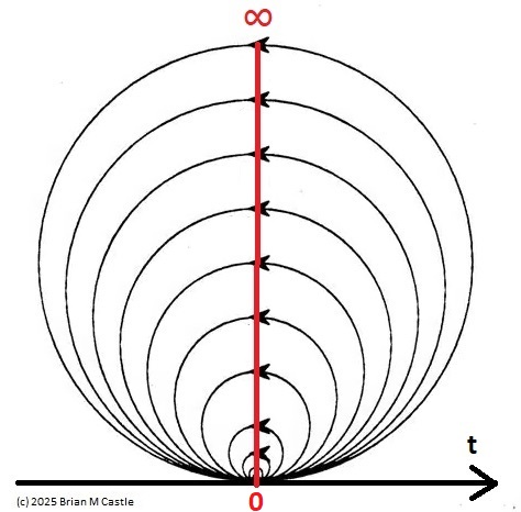

On an earlier page we noted the geometry of signals related to a voluntary motor action. If we take this orientation and map it onto the compactified timeline, the direction of travel is always maintained consistently around the loop, and the part we're most interested in is the point at infinity, because this is where sensory input becomes motor action. (Consider that concept in the broadest possible sense, especially in the limit as dt => 0, where there is involvement of both the real-time information model and molecular processes related to memory).

Having seen the earring, we notice that all the points at infinity directly apposed to T=0 are aligned in a straight line, and the radius of each loop corresponds to the processing window of the underlying timeline. The plane of the earring can then be mapped onto a (possibly non-Euclidean) manifold for optimization purposes, and any such embedding will necessarily process the joint distributions across the timeline. This way predictions are correlated with outcomes at multiple levels of resolution, and these relationships can then be conveniently reorganized for computation.

To emphasize, the radius of a loop models the length of a reflex arc. A reflex arc is viewed in the broadest possible terms, as a directional signal flow that can occur at any level of resolution. There are reflex arcs in the ordinary (anatomical and electrophysiological) sense, and there are also reflex arcs at the molecular level, and at the level of entire neural networks and subsystems. These loops have two things in common - they all intersect t=0 "now", and their points at infinity all line up in the compactified space.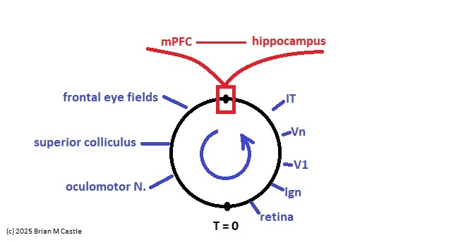

Already, when viewed this way from a whole-brain standpoint, it makes sense that the areas near T=∞ that close the loop on the sensory => motor connection, should be the same areas involved with memory, and thus the same areas involved with the modeling of T=0. Returning to an earlier diagram, we see that this is indeed the case - the circuitry around the hippocampus and prefrontal cortex that lives around T=∞ is the same circuitry that handles episodic memory, and it's the same circuitry that handles spatial-cognitive mapping.

Note that the projected (compactified) view extends beyond the boundaries of the linear timeline (the green line, in the figure below - we got this when we added the point at infinity). However the resolution of the neighborhood around T=0 is considerably greater than that near the boundaries. The compactification has given us an almost "foveal" insight to the area we most need to decipher in a real time setting. And note that the neighborhood of infinity (the point labeled "observer" in the drawing) is precisely the area where we wish to place the hippocampus and prefrontal cortex, based on the earlier discussion of the stylized timeline.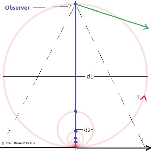

The neural timeline can be considered as an extension of a time series in which future points are predicted. Predictions become constrained (and therefore one hopes more accurate) as we move leftward along the timeline from T >> 0. In this sense each neural network layer along the timeline acts like a Kalman filter, predicting the next network state from the information within a moving window. This idea dovetails quite perfectly with concepts from machine learning like predictive coding and energy minimization.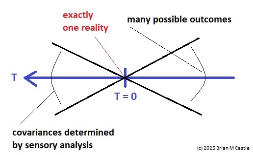

The idea in the earring, is that predictions are matched with outcomes, at many different scales and at many different resolutions. If we really wanted to trace the path of an action potential through the network, we would end up with a very nonlinear Kalman filter that would have to be described in terms of Volterra kernels and beyond, and such an exercise while interesting is not necessarily useful. But we can loosely conceive for example, a situation in which a voluntary motor action is staged along the timeline and then modified by ongoing sensory information. At the far right of the timeline, there are many possibilities for the actual outcome, but as we move inward, sensory conditions are processed and the range of possibilities is narrowed, until at T=0 one sensorimotor reality is materialized.

A complete mathematical description of the earring topology is beyond the scope of these pages. It is well studied, including its fundamental group and its embeddings (de Smit 1992, Eda and Kawamura 2000). (The information is readily available online, with a simple Google search). Here for example is an earring considered as a cross-section of a toroidal spiral.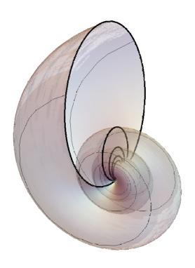

Note that in the description above, the origin is implicitly defined as the intersection of the circles that make up the earring. But we've already seen, that the origin is arbitrary - we can move it anywhere. With a simple rotation, we can move it to the opposite side of the circle, directly opposite the intersection of the hoops. After talking briefly about the ability to resolve individual points along the timeline, we'll see that with the proper embedding, we can even move the origin inside the circle. Embeddings are introduced on the next page.

A Practical Application

Setting aside for a moment the issues around the neighborhood of infinity, here is a practical application of the compactified timeline (especially if you're a stock trader). We can do multi-window Granger causality analysis on any two compactified time series taken from the timeline, by simply rotating the circles. Here is a schematic of the underlying calculations. Look familiar?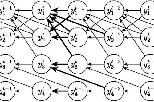

Causality analysis involves sliding the two time series relative to each other, which in the compact space becomes a rotation. When appropriately embedded, the output of the compactified network results in maps like this (and note that these are relationships in time, each arrow represents a correlation with a particular lag - for example if this were the stock market we might be interested in the one way arrow between livestock and supply shock, indicating both the relevant delay, and the corresponding correlation or likelihood).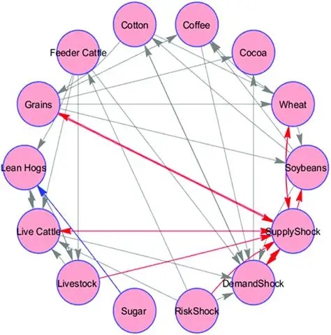

Instead of market data though, in our case the circles will attach to points along the timeline, and we'll be extracting "micro-causality" in real time from this network. We do not make the assumption that causality is stationary, instead we learn to identify and exploit the non-stationarities. If you're a stock trader, you can do this in real time with a neural network, you don't have to wait overnight for an analysis. You can take your nVidia GPU with you to the trading floor. ;)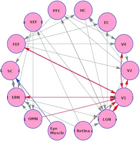

In a human brain, the idea of weighted connections along the timeline becomes closely related to real time abilities. In a biological context "real time" is mostly defined by the environment, in other words the organism is optimized to be effective in its environment, and it doesn't have to exceed that unless there is a specific need. However in the timeline model presented here, "real time" has a deeper meaning. The model is topologically self-similar, which means real time should extend all the way to the limit as dt => 0. This means "environmental speed" is no longer adequate, we need faster processes. If we want to get down to the range of molecular kinetics, we need at least microseconds - the milliseconds from a neural action potential aren't quite fast enough. Before expanding this model, it helps to have an idea of the range of time scales in play. Many scientists think of neural activity in terms of milliseconds, perhaps seconds, and this range is likely reasonable for single neurons. However neurons in populations acquire considerably better resolution, and this becomes vitally important in the consideration of asynchronous information processing architectures.