What about those graphs? We've seen a couple of versions of them already. One version was algebraic, involving vertices and edges. Another version was dynamic, involving optimization on energy surfaces where the location of the minima are related to dynamic attractors.

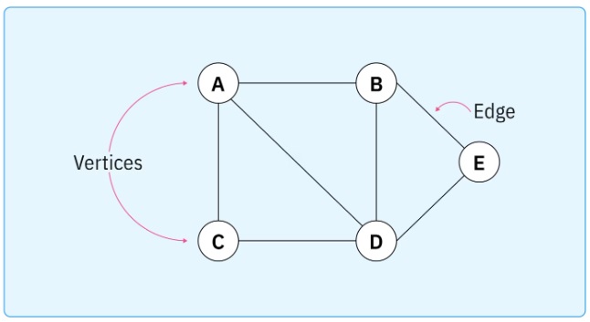
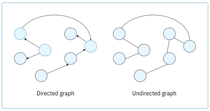
In its most basic form a graph is a set, and a collection of relationships on that set. This structure can be used for many things, including the elaboration of motor behavior during navigation, and the cognition related to the solution of working memory tasks. Graphs can be either directed or undirected.

This figure shows the adjacency matrix, which is fundamental to graph structure.

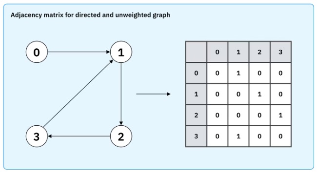
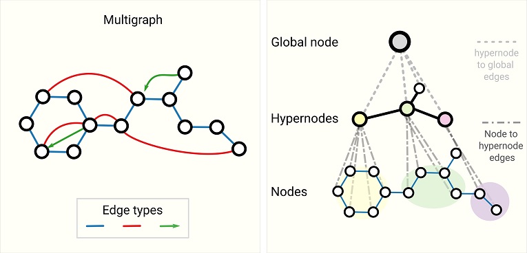
To translate a graph into a neural network, one can load the adjacency matrix into the synapses. In a Hopfield network, this will guide the dynamic to the individual attractor nodes. The network can be programmed to produce either the whole graph or the set of (possibly directional) connected nodes. The adjacency matrix will generally change over time to reflect evolving relationships, that's part of the learning that occurs with dynamic spatiotemporal graphs. In modern machine architectures the spatiotemporal block adjacency matrix is combined with transformer architectures that predict missing temporal links. This method has realized accurate albeit highly non-biological networks. The key steps in this method are first, the generation of regional adjacency graphs and their combination into a block adjacency matrix, then projection into a higher dimensional space followed by application of the transformer, next a smoothing pass that encourages symmetry and sparsity, and finally the mapping into the GNN that enables classification and prediction. In the machine learning world there are all kinds of non-biological architectures, as shown in the figure below. These types of relationships are more naturally represented in terms of information geometry, as dicussed on these pages.

In a machine learning context, the things we watch out for include zero Laplacian eigenvalues, and low Fiedler values. The Fiedler value is the second smallest eigenvalue of the Laplacian matrix of a graph. The Laplacian of a graph is also called its admittance matrix or its Kirchhoff matrix. It is defined as follows:

L(G) = Δ(G) - A(G)

where A(G) is the adjacency matrix and Δ(G) is the diagonal matrix whose (i,i) entry holds the degree of the i-th vertex of G. The graph Laplacian is a positive semi-definite matrix. The dimension of its nullspace is the number of connected components of G. Graphs can easily be represented in Hopfield networks (Rao et al 2026). In large graphs we're interested in the spectrum of the Laplacian, which can be extracted in a size-invariant and scale-adaptive manner to support comparisons (Tsitsulin et al 2018).

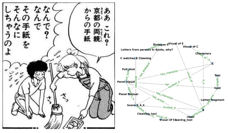
Why use graphs? Isn't object recognition enough? Well... graphs represent much more than just simple object relationships. For example, a graph can be used to represent physical relationships. A cup can be balanced precariously on the edge of a table, or a running dog can temporarily disappear behind a tree. Graphs represent physical scene understanding. Scene graphs are an important area of current research in machine learning. Scene graphs represent complex relationships hierarchically and topologically, enabling structured reasoning in addition to simple object detection and mapping. Hierarchical knowledge graphs are important for the understanding of "stories", which are like unfolding visual scenes (Chen 2025). The figure shows the translation of a visual scene into a knowledge graph. Look familiar?

This figure shows the same thing for sequence relationships.

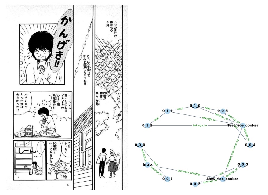
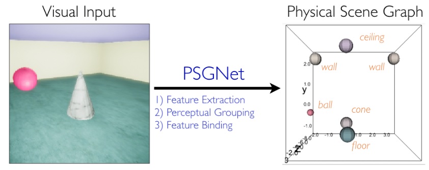
The primitives labeling the edges of the graph include things that can be phase encoded, like the relationship "precedes", and the relationship "next". Other relationships may not be directly derivable from the visual scene, and instead must be pulled from memory as "context" (this might include the primitive labeled "belongs_to" in the graph). The figure below shows a simple machine learning model of graph building from a visual scene. First the relationships are represented, which in the visual system depends on the extraction of retinotopic features, the perceptual grouping of visual elements into objects, and the binding of features to objects.

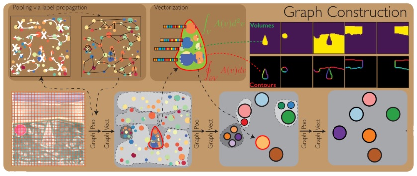
Next the graph is built. You can see on the bottom left of the figure, a geometry that resembles the hippocampus and entorhinal cortex, with a structure that can be interpreted as a collection of grid cells and place cells.

In some cases a graph architecture can be built directly into the neural network. This is the approach taken by Burns and Fukai 2023, who wired Hopfield networks into simplicial structures. This approach changes the network dynamics, as does making the connections recurrent or asymmetrical (Xue et al 2025). In many cases the distance between two nodes in a graph can be entirely separated from the values and properties of the edge (Zhu et al 2021).

The need for graphs in neural networks includes the attention function, which can be considered a regulatory mechanism related to working memory. In the machine learning world, a "graph attention network" assigns learned task-dependent weights to neighborhood nodes during feature aggregation. Unlike graph convolutional networks, graph attention networks do not require a fixed graph structure, and thus perform well in tasks like node classification and graph representation. Graph attention networks have an inductive ability, they can predict representations for previously unseen nodes or entire graphs. Such networks have been used for example, for visual imitation learning (Sieb et al 2019). In a graph neural network, object relationships generalize to things like language binding (T Le et al 2021).

In spite of the complex vocabulary generated by a combination of neuroscience and machine learning, the basic idea behind a graph neural network is straightforward. We want to represent the graph on the left, in the neural network on the right.

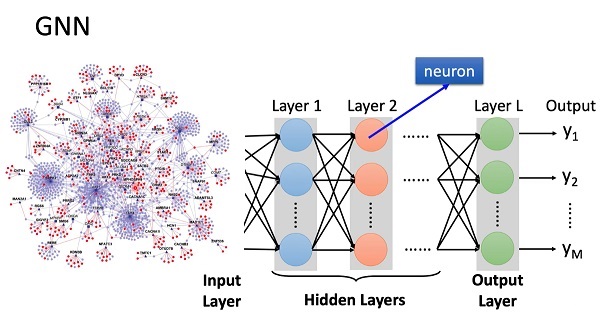
You can see the problem. The graph gets complex, real fast. We're trying to represent a complex graph in a small neural network. There has to be a better way. Parameterizing the information is one way. Bayesian relationships though, are generally high dimensional. In any number of dimensions, there is no guarantee that any particular collection of nodes and edges will be separable. We need a flexible architecture that lets us restructure the information on demand.

In a visual field, the first task of analysis is to separate figure from ground, to individuate objects in terms of their structure and the consistency of their motion. In a human brain, this capability self-organizes during development, and becomes mostly hard wired during adulthood (although still plastic). From the visual field to a scene, there is a tremendous compression of information. 126 million pixels in the retina become a few objects in the scene, with distances and angles from the organism, and perhaps with a few properties attached to each object. Events are perturbations, they're things happening to objects, like appearance, disappearance, or motion possibly resulting in a change of relationships. Objects are timeless, but events have a sequence. Events are like "operators", a sequence of events rearranges the objects. The sequence of events is encoded into the phases (delays) of spike trains relative to an external rhythm or ramp. The location of objects is topographic, which is a different axis of representation from the events that end up as sequences of spike trains. In early vision, the location of a spike train in the topographic network signals the location of an object, but in the scene map, this gets converted into the phase (delay) of a spike relative to an internal coordinating signal. This frees up the topography, for use in some other purpose. And in fact it is the brain itself that's mapped into the hippocampus, not the topography of the visual field. The topography of the visual field ends up being phase encoded, by wavelet transforms that represent both spatial and temporal information.

Wavelets are ideally suited for converting sequence information into graphs. If information can be encoded by wavelet phase, then local credit assignment can be recovered simply by looking at earlier spikes in a spike train, and that is exactly what we see in the working memory in prefrontal cortex. Earlier events are encoded as earlier spike in the spike train. So if spatial position is encoded in the spike train, and temporal sequence is also encoded in the spike train, what does that tell us? The answer is the encodings happen in different neurons. Both neurons have similar spike trains, but one is encoding spatial position and the other is encoding temporal sequence. That means downstream, spatial position becomes the same as temporal sequence. This is a spacetime encoding, not just a space or time encoding. It's using a different geometry, one not related to the topography of the visual field. The spacetime concept kind of leaps out at us, doesn't it? Like, in relativity, with its Minkowski metric and its hyperbolic geometry and its curvature of the spacetime manifold. What would happen if we could represent information this way? Events on a light cone make a great deal of sense, don't they? There are ordinary events, and impossible events, and events that happen to fall exactly on magic lines called "geodesics". What's up with that?

We can begin by looking at information in a slightly different way. Not just the information itself, but specifically the representation of the information. How do you parametrize it, so it can be easily accessed in a graph-theoretic framework, while at the same time being accessible to geometric manipulations? That is the subject of information geometry, which we'll look at next.