We already talked about the idea of "hot spots" in a visual image. Let's say for the sake of discussion, that these spots are associated with objects in the visual field. We can imagine that the center of a hot spot corresponds with the center of mass of a visual object, and its extent corresponds with the object boundaries. Within this hot spot, the visual system can encode the entirety of the information about that object. In the parallel systems of the visual cortex, we can extract luminance and contrast, color, spatial frequency, motion, binocular disparity, and a lot of other information. Even special purpose information related to things like faces, for social interaction. In this model, the location of the hot spot is the location of the object. In the scene map, only the location of the object has to be maintained, its characteristics can be maintained elsewhere. What's important for the scene map is only the identity of the object and its location, and the things that happen to it. An object can be "tracked" in the visual field simply by adjusting the location of the corresponding hot spot. Tracking of objects is a function of the scene map, as is the attention associated with the tracking.

A hot spot is a "phase transition". It's a different processing mode, a different phase of matter. Just as the ferromagnetic dipoles lose their alignment with heat, a patch of neural network can stop oscillating when the input goes away, or it can start oscillating at a different frequency which will make it lose coherence, possibly causing the entire dynamic assembly to decouple and fall apart. It's easy to create dynamic assemblies in a neural network, the real question is what they're good for. What computational powers to dynamic assemblies bring to the table, that couldn't be accomplished without them? One of the answers lies in the processing at and around the critical point. The critical point is where decisions are made, when oscillators decide to join or not join a dynamic assembly.

It is important for neuroscientists and students of machine learning to understand the Ising model of ferromagnetic behavior. It begins with a simple lattice of "nodes", which in our case we consider to be neurons. In the real physical case of a ferromagnetic material, these nodes would be atomic magnetic moments, spins that point either up or down. In the simplest case they are binary, but in a more interesting case they could take on analog values.

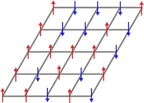
As we raise the temperature, the dipoles start to disalign, and we get fractions of them that are at this angle or the other. We can calculate (approximately) how many of them are at a given angle using statistical mechanics. In the extreme situation, all the angles are random and there is no relationship between any of them, however there are situations in between where there may be pockets with a greater ratio of one angle or another. In this case, we are interested in the relationship between these pockets, because Kuramoto tells us that when oscillators of the same frequency interact, their phases tend to couple.

Instead of raising the temperature to decouple the oscillators, we can also do the opposite, we can begin at a high temperature with a fully decoupled system, and then lower the temperature so the magnetic dipoles start aligning. This is roughly what happens in a Boltzmann machine, the temperature gets lowered until there is some form of alignment. In this case we're interested to know whether there are any interactions between the dipoles - in other words, does the alignment of dipoles in one region somehow assist or hinder the alignment of dipoles in a different region?

In the original Ising model there was no concept of "oscillator", there was simply an angle attached to every dipole. To get an oscillator, the angle has to move back and forth like a pendulum. This formalism is easily introduced. The figure shows a network with oscillators, tied into a mesh with resistors.

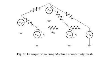
In an "Ising model with oscillators", or "oscillator based Ising model", resistively coupled nonlinear oscillators represent the spins, and the system dynamics are represented as differential equations in the oscillator phase, much like the Kuramoto approach. Such systems admit a Lyapunov function that matches the Ising Hamiltonian at stable equilibria, which in turn allows the system to evolve to its lower energy state. Oscillator based Ising models show dramatic performance improvements over phase-amplitude models for combinatorial optimization problems (like the traveling salesman problem, or planning a trajectory to reach an object in visual space). So how does a spin lattice relate to information processing?

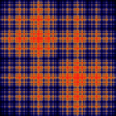
The original Hopfield network was based on the Ising-Lenz model of ferromagnetic behavior (Ising 1924). Each neuron, in a Hopfield network, represents a spin state in a lattice. The spins are either up or down (1 or -1), corresponding to the states of the neurons. The synaptic influence experienced by a neuron is like the "field" experienced by a spin state in the Ising lattice, in terms of its contributions from all the other spins, and possibly from a bias term usually represented as b, that could be related to an outside field. For information processing purposes, we are interested in the transition probabilities of the spins, from one state to another (because if we can control these probabilities, then we can store and process information). These transition probabilities are what a Hopfield network manipulates. At each tick, when a neuron is selected for update, if the direction of its spin matches the direction of its field nothing happens, but if the spin is opposite to the field then the bit will "flip" with a certain probability, just like the noisy quantum spins in a ferromagnetic lattice. For example in this figure the transition probabilities are shown in orange. Clearly, there is a geometry to them.

More specifically though, we're interested in the "order" in such systems, and particularly in the long range order. This concept is necessary to link the Ising model with nonlinear thermodynamics, which we'll look at on the next page. The order parameters relate to the "coupling constants" between oscillators. Also important for us to understand, are the boundary conditions, both globally and locally. This seems a bit of a tall order, but much can be learned with just basic statistical mechanics (like the Gibbs formalism).

So what's the deal? Why are we talking about spin states in a section about information geometry?

Information Geometry

Information geometry ties together many of the concepts we've already looked at. For example it admits cost (energy) functions in the form of Lagrangians that can be directly tied to dynamic behavior and optimization architectures. The bit configurations in a Hopfield network are a tiny subset of this consideration, but it's useful to ask another question, in the context of large modern Hopfield networks, which are flexible and powerful and can be used as hierarchical associative memories. The question is: "where do we put all that data?" How do we organize it? We looked at graphs, and quickly came to realize that graph architectures get complex, just due to the sheer number of nodes and vertices. Information geometry provides a different way of representing data, in the form of manifolds, little surfaces that together form bigger surfaces. Information geometry gives us math to deal with these structures. It uses the tools of differential geometry to organize information in a mathematically useful form, with common representations that apply to every kind of network architecture, from convolutional to recurrent to the real-time map we talked about in the first sections.

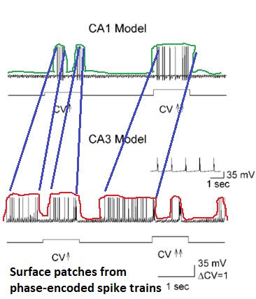
Information geometry is the science of separability. It's also the mathematics of representation, and parametrization. Separability is a big deal in machine learning. Perceptrons can perform linear separability, and related architectures can handle some nonlinear separability, but what is it exactly that confers separability? Data scientists use tricks like projecting the data up into a higher dimension, so axes that might not have been predefined become visible. If we had a perfect correlation engine so we didn't have to know any categories or relationships in advance, how can we best represent the data so that related information is clustered together, and unrelated information is separable? And how can we then zoom in, in such a way that the clustered information becomes separable too? One of the interesting things about the kind of phase encoding that happens in the hippocampus, is that the resulting spike trains end up resembling little surfaces. If one were to draw a curve around the shape of the spike train, and then combine several such curves, one would obtain a surface. That is to say, a small "patch" of surface - a mini-surface.

The basic concept in information geometry is an "information manifold". This is a parameterized "shape" that's usually represented as a surface in an embedding space. To be computationally useful it should be a Riemannian manifold, that is to say, it should have an inner product so we can define distances and angles. Information geometry uses many of the same concepts as differential geometry, like connections that preserve the inner product. The information manifold is made of points, that are pieces of information. This is a broad concept, as we'll see shortly. The information manifold induces a "metric" on the points, that is to say, a way of defining the distance between any two points. We can thus draw paths between the points, and geodesics that represent the shortest distances. One can also imagine that each path has a probability attached to it. On the surface this becomes a "probability field", a tensor. Each point on the surface has a tangent plane (relative to the embedding space), designated in the usual way as TpM (the tangent plane to the manifold at point p). The collection of such tangent planes is the "tangent space", which has the same dimensionality as the manifold itself.

The entirety of differential geometry is beyond the scope of these pages. There are plenty of excellent resources online, and on YouTube. Every biologist should be familiar with these concepts, they are basic and fundamental to the study of neural networks. In differential geometry, there are two ways of looking at things, the intrinsic view and the extrinsic view. The extrinsic view is a lot easier, we can move things around on the surface using parallel transport, the same way the physicists do. This method uses the Levi-Civita connection between the tangent planes to define a metric tensor at every point in space, which is then used to calculate the dot products. However in the intrinsic geometry, we're not allowed to use normal vectors that point up above the surface, we're not allowed to use the embedding dimension. All our integrals have to be along paths intrinsic to the surface. We are in effect living in Flatland, in the interior geometry. Both approaches are useful, and we should be able to freely translate between them. Of course, a key question becomes what exactly constitutes the embedding dimension, and we already started answering that question in the first few pages - it's simply another neural network. (Our brains are embedded into themselves! Commissural connections pretty much guarantee that at any given moment there will be some kind of "observer" hovering around the point at infinity).

Speaking of points at infinity... we saw how compactification can result in Riemann spheres, "projection mappings" that turn lines into circles and circles into even more complicated geometries. We also touched on the idea of a space-filling process, one that covers a timeline at multiple levels of resolution and relates the windows by comparing models of the current moment. All these things can be represented in terms of information geometry. The question is, how do you organize the information? Where do you put it? If you just willy-nilly start creating graphs in a neural network, they get very unmanageable very quickly. An Irish setter is related to a golden retriever, but only during the week when the dog show isn't happening, the rest of the time they're on a leash and they have to behave. They're both dogs... but what a complicated set of concepts! Dog shows, leashes, and what does "behave" mean? If you tried representing all this as a graph, it would result in what the programmers call "spaghetti code", more threads than a spider's web, making it impossible to find the center. So there has to be a better organization to the data. Part of the process of memory consolidation is making sure the data is organized in the best possible manner. This suggests we're moving on from a phase code, we're transitioning into something else - something that takes time to figure out, because consolidation takes a hundred times as long as a scene. In information geometry, the process of consolidation involves organizing the mini-patches into larger surfaces. Topologists approach this issue with charts and maps, which lets us build connections from one tangent plane to another. In a Hopfield network, the information is represented as an energy surface, and the energy is like a ball rolling down the surface, trying to find a minimum. Any such surface can be lifted directly into an information manifold, and the tools of geometry used to reorganize the information. The idea of "training" a Hopfield network by creating a set of attractors thus takes on a new meaning on a larger manifold.

A bit flip in a Hopfield network is like a tiny movement along an information manifold. Before, your network state (and transition matrix) was over there, now it's over here. The path taken between the two parametrized points, is a "ds" along a curve, and in a gradient descent network it's usually along a geodesic. If one were to phase encode the entire time sequence of Hopfield output during training, one could visualize the paths taken by the representation of the information - that is to say, the development of energy wells and attractors. This is only one of the many powerful applications of information geometry.

An interesting thing about the visual system is that everything is two dimensional. Everything is retinotopic, until we get to the object recognition areas, and even those look like they're at the end of a convolutional stream. But the rest of the brain isn't necessarily two dimensional. The auditory system is basically one-dimensional until it gets to sound localization, whereas the somatosensory system is inherently three dimensional, as is the entire sympathetic and parasympathetic apparatus. There are definitely three dimensional organizations in the brain. The striatum is likely one of them. There are different geometries conferred by three dimensional compactifications, than two. Compactifying a three-dimensional volume into an embedding space results in a four dimensional entity. Some things are possible in four dimensions, that are not possible in three - and vice versa. For instance there is no "cross product" per se in 4 dimensions, because the concept is ambiguous. A very instructive use of information geometry is its application to the retina in the early visual system, which seems like the world's simplest neural network. It only has a few layers, and it doesn't even have any recurrent connections. Of course... we already looked at it, it's more complex than it seems. But scientists... how can I say this... they're still futzing around with receptive fields. What's being taught in medical schools today, is receptive fields. What they should be teaching, is information geometry. For instance - in a wonderful theoretical paper, Ding et al (2023) explain the applications of information geometry in the retina.

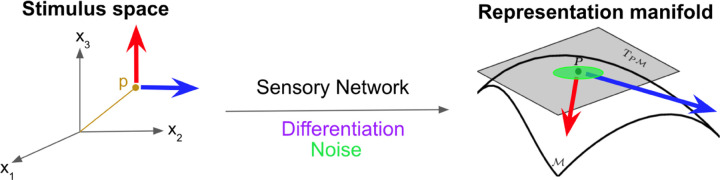
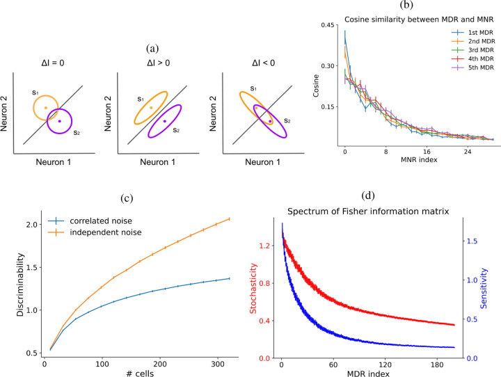
In this figure, the sensory network maps from the stimulus space to the representation space, and the differentiation operator maps one tangent space to the other. Here the effect of noise is shown in green, and the red and blue arrows represent sensitivities, which are directional because they're related to the basis on the manifold. The motion of an image on the retina induces a "most discriminable direction", which is actually encoded in the receptive field but is almost never tested as such in biological experiments. The most discriminable direction in the retina is too fast to be tested psychophysically, and it's even doubtful whether it enters perception. However it's definitely testable in a live recording situation. This model predicts not only the most discriminable direction of motion at any point in the visual field, but also establishes definitively that correlated noise is detrimental to retinal processing, invalidating dozens of models that attempted to invoke correlated noise as a mechanism underlying non-local coupling in retinal receptive fields. Instead what we have is a subtle and temporary shift in the shape of the receptive field so as to give it a "preferred direction", which is induced by neighboring neurons. This is a superb and insightful application of information geometry, even though it's a simple example it reveals the power of information geometry as a tool for understanding neural networks.

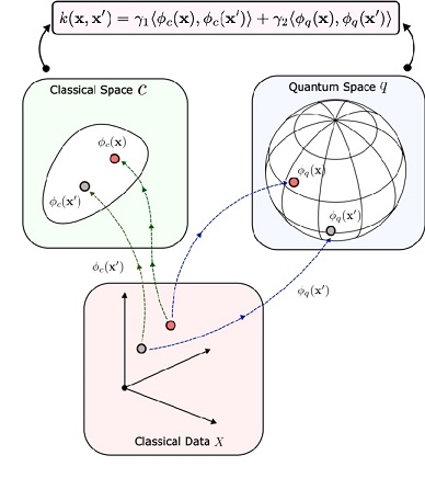
Information geometry has another set of roots in information theory. We already looked at some information theory in the form of the Shannon entropy, and the von Neumann entropy. In Bayesian inference, which underlies a big fraction of modern AI, beliefs are represented by parameters, that are updated whenever new information arrives. Beliefs are estimates of the relationships between things, given a current context. The relationships between things are points on an information manifold, and distances between them. As the beliefs change, the points move around, and the distance between them changes. Beliefs are represented as probabilities, and to update the Bayesian parameters we need a bidirectional mapping between the data and the parameters. Information geometry provides us with exactly such a mapping, in a computationally useful form, from which we can derive geometric structure and symmetry structure (Lie groups apply directly to information manifolds) and a host of other useful information that lets us compress data and access it in a useful way, enabling powerful capabilities like the "zooming in" we talked about. In information geometry, the points on an information manifold are statistical distributions, they're probabilities. The distance between points is given by the Kullback-Leibler divergence, which measures the information difference between two distributions. The KL-divergence is related to the Fisher information metric, which characterizes the local discriminability of information (in this case, stimuli). The figure shows an example of the the lifting of a dataset onto a Riemannian manifold. This is an important example because of its relationship to quantum computing, which we'll touch on very briefly at the end of this section because it's related to the upcoming technological explosion in photonics.

Information geometry "can" be computationally intensive. Rearranging patches of a manifold requires at minimum the solution of the Jacobian and Hessian matrices for every point in the mapping. However we don't always need to perform such radical surgery, sometimes we have simpler needs. And in a real brain, simpler is better, because it's faster.

Next we'll take a look at information geometry in the context of dynamic activity. Esentially we'll be looking at the information geometry of the Belousov-Zhabotinsky reaction, where there is an oscillator at every point in space - a situation that closely resembles a neural network!