The thermodynamic approach to neural networks begins with the work of Lars Onsager, who solved the transition matrices for simple Ising systems. A milestone was reached in the 70's with the work of Ilya Prigogine, who used nonlinear nonequilibrium thermodynamics to understand reaction-diffusion systems. Along the way, there was a considerable amount of work in probability theory, like the Ornstein-Uhlenbeck process that describes mean-reverting generators (of the kind one might find in driven neural oscillators).

We already looked at the Belousov-Zhabotinsky reaction, which is an example where there are oscillators at every point in space, coupled through long-range interactions. It turns out, that the Belousov-Zhabotinsky dynamics can be used for computation, just like the Hopfield network uses Ising dynamics (Toth et al 2008, Gorecki et al 2014, Rambidi et al 1998). The idea of using nonlinear thermodynamics for computation is not new, it's a simple extension of the Gibbs formalism for equilibrium statistical mechanics. However its application to neural networks is definitely new. To my knowledge as of this date in early 2026, it hasn't been addressed yet, neither in neuroscience nor in machine learning. So let's address it!

To begin with, there have been plenty of hybrid models involving both convolutional networks and Hopfield networks, but they've been built for the purpose of image recognition and classification against canned datasets (like the MNIST standardized training sets), therefore they're built on serial architectures. To date there is nothing like the timeline architecture proposed on these pages. Compactification exists, but it's used in specific ways not necessarily related to the fundamental topology. To date there is no model that I know of, that uses the Hopfield "thermodynamic" architecture transversely across a serial network. Part of the reason is because it's a real-time architecture, its goal is different from most machine vision tasks. So let's address this too - we'll address both issues at the same time.

The thing to realize about the brain, is it's an open system. If we're talking about statistical mechanical systems (I call them "thermodynamic" networks), assumptions are frequently made regarding the closure of the Hamiltonian (or equivalent energy function). Machine learning engineers are well aware that these functions change over time - in addition to the energy related terms in a Boltzmann machine and the information related terms in Friston's version of the energy function, there are terms related to the outside environment, for example the relationship of self to others and to the world. These may include things like emotional bias, and its interruption triggered by the sudden appearance of a predator. In the brain, there's not really any such thing as "equilibrium". Everything is constantly changing, there isn't enough time for equilibrium. Certainly there are equilibria, but the information flow isn't necessarily a part of them.

Non-equilibrium thermodynamics is a thorny subject. For one thing it's complicated, and for another, a lot of assumptions have to be made to get any mathematical tractability. Nevertheless, the B-Z reaction is an excellent example where those assumptions result in a reasonably accurate description of a real system. In a computational context, the idea is much like a Hopfield network, it's to control the activity at a particular point in space. In a computational B-Z network, space becomes discrete and the oscillators are embedded into a lattice, just like the spin lattice shown on the previous page. The connections in the network are the couplings between the oscillators, a design we can apply directly to the Kuramoto model. It turns out, that the coupling constants between oscillators can be learned adaptively, synaptically, just like those in a Hopfield network. In this concept, each oscillator is a neural "module", a small network wired into a motif that supports multi-stability (perhaps like a mini-column in the cerebral cortex). This type of architecture has been investigated in many ways by many people, for many purposes. Examples certainly abound in the simulation world, you can find some in the Nest examples referenced earlier. Some of these networks are very close to what we want, in terms of an embedded timeline. The cortical architecture certainly fulfills the basic prerequisites for mutual embedding, there is vertical modular connectivity and parallel connectivity between modules. If there is any "equilibrium" in such a system, it is rapidly perturbed by the input. The environmental input is constantly driving the brain, and in turn the brain has systems that handle equilibrium conditions in some sophisticated ways, for example the resolution of a delayed reward scenario.

The relationship between a network of B-Z oscillators and an information geometric manifold is straightforward. A B-Z lattice is basically a three dimensional version of an Ising lattice. All that means is, there is extra dimensionality in the information manifold. What does it mean to "oscillate" on an information manifold? There are already examples of Hopfield networks built with oscillators (Cai et al 2025, Cheng et al 2025, Al-Kayed et al 2025).Such networks display all of the basic behaviors we've been discussing.

We can simply extend these two-dimensional oscillating Ising networks to three dimensions, and that should give us a pretty good idea of the behavior. We should be able to model this configuration on any decent simulator. One thing we would certainly like to investigate is the relative timing of the embedding network and the timeline. Another important issue is the multi-stability of every point in the embedding network, and the relationship between that and the information flow along the timeline (we already covered part of that with phase encoding, but there's certainly more to it). To investigate these things we first need a timeline that behaves, that is to say, it stays within a useful computational range. So in a modeling effort, dynamics should come first, the network has to support the required dynamics in all its variations. After that we can investigate which synapses we should make plastic and in what ways.

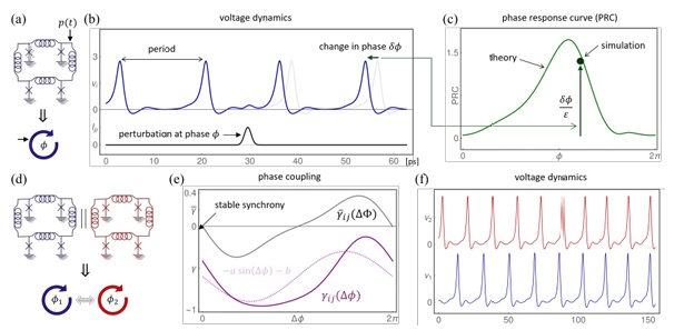
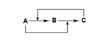
Returning to the lattice of oscillators, we have a situation that has never been fully explored in the theoretical literature. We have what basically amounts to a Kuramoto model, however all the oscillators are at different frequencies. They're not just multi-modal, their frequencies actually vary over time, both in real time and in terms of the synaptic plasticity that regulates their coupling. The figure below shows the basic scheme of a B-Z reaction, the arrows indicate the coupling between volume and rate, so for example the amount of C determines the rate of the reaction from A to B.

In a neural network we have a much richer spectrum of couplings. This spectrum is determined by the connections along the lattice. For example in the primary visual cortex where the diameter of a mini-column is around 100 microns (0.1 mm), axons from within each module may branch in the 2-3 mm range around the node. So if we're trying to model a "patch of cortex" we need a fairly large patch, there should be several such overlapping hypercolumns and each one consists of 20-30 mini-columns along an axis (so about 400-900 in total). This is a large model, in a grid consisting of three neighboring hypercolumns it amounts to a little under 18 million neurons, even if we reduce an oscillator to just 2 neurons instead of the 100 or so typically found in a mini-column. There are very few simulators that could handle such a network. It can (and has) been done on an IBM supercomputer, at scale. Unfortunately today's FPGA chips can only handle 100,000 neurons or so, but they're getting better quickly. They're commercial efforts, they scale according to commercial need. As the demand scales, so do the chips.

Let's consider the "asynchronous update" requirement in a Hopfield network. Does this also apply to a network of Kuramoto oscillators? Well... yes. The oscillators should not be updated synchronously, and therefore we have the thorny problem of running Monte Carlo simulations in multiple dimensions for 18 million neurons. :( The random number generation alone will bottleneck our simulator unless we have specific hardware dedicated for that purpose, and such hardware is expensive and difficult to obtain. So what can we do? One thing we can do, is simplify the coupling between the oscillators. The lattice has a regular arrangement, therefore so do the connections. If we can specify a distance measure in the lattice, we can approximate the connectivity using the distance, and in multiple dimensions where the connectivity changes all the time this becomes the "shape" of a geometric transform - and we can change the shape using the synaptic weights. These calculations amount to drawing from a distribution. The shape of the distribution is changed by the synaptic weights. This is a very simple task for a neural network, it's actually an elementary first-year form of machine learning! It's nothing more than the Bayesian updating of a distribution based on incoming evidence. So that's how we couple our oscillators, and make them adapt to our input. This is "one" way to engage the coupled oscillators for computation.

If there is a generalized oscillatory pattern across the network, the downstream result is a collection of spike trains that encodes the pattern. When this collection of spike trains is phase encoded against external theta (a "much slower and topographically specific waveform"), the phase encoding will extract the local temporal relationships between the spike trains. Thus the population as a whole will come to encode the topographic pattern of the oscillations. From there, the information becomes just like any other neural information, it can be memorized, used for adaptive computations, and so on. These forms of representation are additional degrees of freedom or "dimensions" in a neural network, they go beyond the 2-dimensional retina and the 3-dimensional binocular visual space. In information geometric terms, when we need to project information up into a higher dimension, this is how we do it.

As a last salvo, let's take a look at quantum computing, in the context of neural networks. The essence of quantum computing is the "qubit", an element with an infinite state space. Just like coupled oscillators, a qubit can be coupled with other qubits, in the quantum world this is called "entanglement". In quantum computing, coupling (entanglement) is a resource. There have been some important results regarding quantum Hopfield networks (Rotondo et al 2018, Kimura and Kato 2025). It's instructive to understand the information transforms related to qubits, and the ways in which coupling is used in quantum computations.