The lower portion of the oculomotor system is an excellent place to consider the behavior of individual neurons as it relates to membrane properties. The oculomotor integrator, in particular, is relevant because the membrane properties should match the time constants we observe behaviorally. One of the interesting questions is whether the system time constants are more related to the membrane properties of neurons, or whether they instead depend on the network wiring and population dynamics.
We will work the oculomotor system bottom-up. First we'll make sure the eyes are moving properly in response to the oculomotor neurons. Then we'll hook in the targeting system in the superior colliculus. Next we'll work on visually guided eye movements, and finally we'll move to voluntary movements. In doing so we'll encounter reflexes that have to work, like the VOR.
So let's begin by looking at the simulation engine called Brian2 (Stimberg et al 2019). This is a very powerful engine, and because it's so powerful, it's slow. But it's pretty accurate, in fact Brian2 is the simulator selected by the fruit fly robotics team. A fruit fly brain has about 140,000 neurons, so that's what Brian2 is handling. In contrast, Nengo will handle 2.5 to 6 million neurons (Bekolay et al 2014, Sharma et al 2016), but it's more restrictive in terms of what it can do with them.
One of the advantages of Brian2 is it will run in a Docker image, which means you can use it anywhere, even on a Raspberry Pi. Its biggest drawback is it makes you write differential equations. Now... differential equations are not all that hard - BUT - they take time away from neuroscience. There is a narrow niche in computational neuroscience for determining the specific properties of individual neurons (it becomes especially important in simple organisms like Aplysia, where feeding and escape behaviors can be generated by stimulating single neurons). However in advanced organisms one has billions of neurons that are divided into classes on a genetic basis, and one can usually infer in advance that all members of a particular cell class behave more or less the same way. For example it's a good bet that all the rod photoreceptors in the retina have more or less the same membrane properties. To the extent that such properties can be elucidated by a simulator, it's possible that specific time constants matter. However in general the methods for step-wise solutions of differential equations don't offer much precision, and they become increasingly inaccurate with bigger step sizes and longer simulation durations. The Euler method is one of the standard canned diff-eq solvers, and the RK4 variant of the Runge-Kutta family is popular because it offers a reasonable and effective tradeoff between accuracy and performance. Most of the time, scientists engaged in simulation are satisfied with a "qualitatively" accurate model. A "quantitatively" accurate model is much better, and in some cases can be acheived, but in other cases it's a tall order (and that's one of the reasons we need good simulators!).
The Brian2 SimulatorBrian2 was created in Europe by a very large team. It can be installed directly from the Brian2 web site. Its Docker image can be found here. Unfortunately the tutorials use the Jupyter notebook, which is unreliable and frequently stops for no reason. However since Brian2 is mostly about writing differential equations, a better user experience can perhaps be had by simply using the simulator inside a Bash shell, and writing Brian2 code directly. Yes, Brian2 has its own language. It has a grammar and a parser. You can write differential equations in symbolic form, and Brian2 will convert them to code. This is a very powerful capability, rarely found in other simulators.
Here is a simple example of Brian2 code. Note the differential equation!
G = NeuronGroup(10, 'dv/dt = -v / (10*ms) : 1',
threshold='v > 1', reset='v = 0')
S = Synapses(G, G, model='w:1', on_pre='v+=w')
S.connect('i!=j')
S.w = 'rand()'
mon = SpikeMonitor(G)
run(10*ms) # will include G, S, mon
In Brian2, differential equations are captured as simple string variables, like this:
tau = 10*ms
eqs = '''
dv/dt = (1-v)/tau : 1
'''
Brian2 is aware of geometry, but not in the ways one might expect. One of its powerful capabilities is multi-compartment neuron modeling, which means that different parts of the axons and dendrites have different membrane properties. (Brian2's implementation is a slightly more advanced version of the Rall cable model discussed earlier). Here is a description of Brian2's interpretation of branching axons and dendrites and multi-compartment neurons.
Now... calculating the firing activity of multi-compartment neurons is computationally intensive. You don't really want to ask your simulator to fully compute 100,000 multi-compartment neurons per tick, you could earn another graduate degree before the simulation finishes. Instead this capability is usually used in very small models, maybe 100 to 1000 neurons or so. It is "possible" to do more, but it starts pushing most personal computers. In a nutshell, one active dendrite is worth two passive neurons, and when neural compartments can spike individually, the resulting calculations are approximately on the same scale as an entire convolutional network in a machine learning setting, per neuron. (It's probably even worse because you can't use GPU's, you actually have to solve the differential equations!)
Let's begin simple. We have two topographic layers of neurons, and we want to connect them using a set of synapses. First of all, we can verify that Brian2 is doing the right thing with our neuron activity. Here is how Brian2 interprets action potentials:
That looks a little weird, but we can verify that the spike times are in fact correct:
And, here's what happens when we add a refractory period:
We can also verify that the synapses are behaving correctly. Here are some EPSP's:
And here's what happens when we add a synaptic delay:
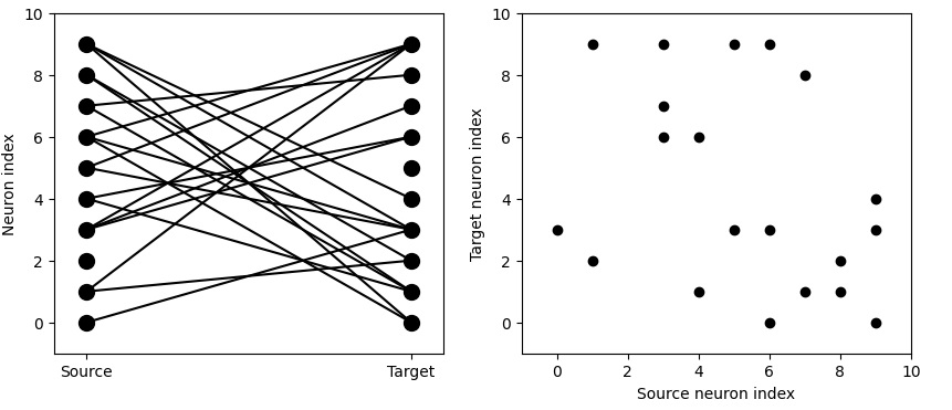
So far so good. Now what about the geometry? Brian2 has a probabilistic connection scheme. You tell it which neurons you want to connect, and with what probability. If you tell it to connect every neuron to every other neuron with a small probability, here's what it might look like:
We're really after something more regular though. We'd like to control our connectivity with probability 1, in many cases. Here's what that might look like:
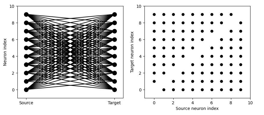
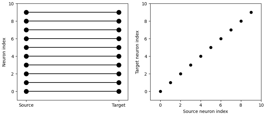
Much better! Now we're getting close to some topography. You can see the delicious line along the diagonal, because we've told Brian2 "i != j". However note that this is not really a 2-dimensional map. You can see the neuron "index", indicating that these neurons are vectorized in one dimension. Can we get something that more closely resembles a two-dimensional receptive field in an orientation column in the primary visual cortex? We can! By telling Brian2 to restrict the extent of the connection.
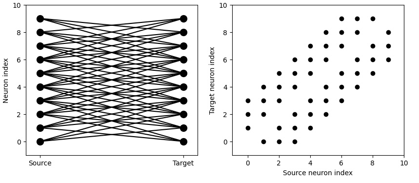
We can get very specific topography with this. We can tell Brian2 to connect neurons 1 to 1 according to their indices.
It's actually pretty easy to get very realistic neuron behavior with Brian2, this way. For instance here's some simple bursting behavior:
Looks pretty good... but is Brian2 capable of synaptic plasticity? Well... let's find out.
Looks like the answer is "yes"! Here's the real problem with Brian2:
eqs_HH_3 = '''
dv/dt = (gl*(El-v) - g_na*(m*m*m)*h*(v-ENa) - g_kd*(n*n*n*n)*(v-EK) + I)/C : volt
dm/dt = 0.32*(mV**-1)*(13.*mV-v+VT)/
(exp((13.*mV-v+VT)/(4.*mV))-1.)/ms*(1-m)-0.28*(mV**-1)*(v-VT-40.*mV)/
(exp((v-VT-40.*mV)/(5.*mV))-1.)/ms*m : 1
dn/dt = 0.032*(mV**-1)*(15.*mV-v+VT)/
(exp((15.*mV-v+VT)/(5.*mV))-1.)/ms*(1.-n)-.5*exp((10.*mV-v+VT)/(40.*mV))/ms*n : 1
dh/dt = 0.128*exp((17.*mV-v+VT)/(18.*mV))/ms*(1.-h)-4./(1+exp((40.*mV-v+VT)/(5.*mV)))/ms*h : 1
I : amp (shared)
C : farad
'''
What the heck is that? Who can read that? Probably the scientist who created it can, but no one else! What does all that stuff mean? Obviously, commenting the code would be of great importance if we chose to do things this way. Another scientist looking at this code might see the name "HH_3" and understand that it's some kind of Hodgkin-Huxley equation. But the rest? Hm... so hit the books and figure out what all the parameters mean, and then there's still the expert knowledge of how to relate the parameters to actual neuron behavior. Many neuroscientists have the expert knowledge, but very few could update the Brian2 code in a couple of seconds or minutes. It would be a lot more helpful to be able to right-click on a cell type or neuron, and update its parameters that way, rather than having to spend hours typing and debugging code.
Generally it looks pretty good though. Brian2 is doing what we want. The main issue from the timeline perspective (besides those nasty differential equations) is the ability to map multi-dimensional geometry into Brian2's neural vectors. Fortunately, the Annie interface tool will take care of that for us. It will uniquely map Brian2's neuron indexes into our own internal geometry, so the simulator doesn't have to know or care where the neurons and synapses are.
Unfortunately, Annie does not currently handle differential equations defined in textual form, nor can it read Brian2's internal functions. The best it can do is export its own internal functions in a form that Brian2 can read. This limits Brian2's behaviors to those recognized internally by Annie. The Annie interface engine has all of the basic functions related to the various model neuron types, and it can set parameters accordingly, however if they are changed inside Brian2, Annie will not pick up the changes. Therefore Annie must "drive" the network definition, if we choose to use the Brian2 simulator.
Looks like, as long as we let Annie drive, we can get what we want. Let's see what we can do with this.
Muscle ContractionThe first goal in this section is to make the eye muscles contract properly in response to interventions in any of the gaze centers. This means we have to map the linearly organized gaze centers into the nonlinear responses of the various muscle groups. Making eye muscles contract is trivially easy in Nengo, you just create an Ensemble that learns eye position (in however many dimensions you need). In Brian2, it's quite difficult, but you have much better control over the behavior of individual neurons as well as the aggregate behavior of the network.
Which simulator you end up using, depends on your goals. In this case, eye muscle contraction is quite precise, the cerebellum gets involved and there is a neural integrator, and saccades are usually pretty much right on target. Eye movements are one of the areas where we probably care about precision, because doctors and scientists over the years have come up with many clever ways to disrupt them or alter their courses in mid-stream. Eye movements are an important diagnostic tool for clinicians, and the responses to perturbation are often a helpful indicator of underlying pathology. So in this case we would wish for our model to be able to replicate the peculiarities and idiosyncracies of real human eye movements, both in the normal case and in the case of pathology.
For the particular simulation we'd like to run here, the precision of eye movements is important. We would like to replicate not only target selection but also the fine points and dynamics around it. So in this particular case, Brian2 might help us, because we'll probably be interested in the time constants around the oculomotor integrator, and the delay time(s) associated with the VOR and so on.
Annie will export code (networks) for both Nengo and Brian2. This way, we can easily compare the two simulators, to see if they're behaving the same way. Let's do that, because muscle contraction is a very easy network, there are a few thousand neurons in the abducens nucleus whose combined activities determine the amount, rate, and acceleration of muscle contraction. We should note here though, that these aspects of an eye movement are conveyed to the superior colliculus through different pathways. The pathways from areas MT and MST in the temporal lobe convey mostly velocity information, whereas the pathway from the frontal eye fields (FEF) conveys mostly acceleration information related to the beginning of eye movements. So, in our model, we'll eventually need to have separate parameters for these pathways. However we can begin by simply assuming that the targeting system in the superior colliculus is working correctly, and this way we can simply provide our model abducens nucleus with a target and a "go" signal. (Is this the way it really works? We'll find out!)
In Nengo, setting up a model abducens nucleus is very easy. The network would look something like this:
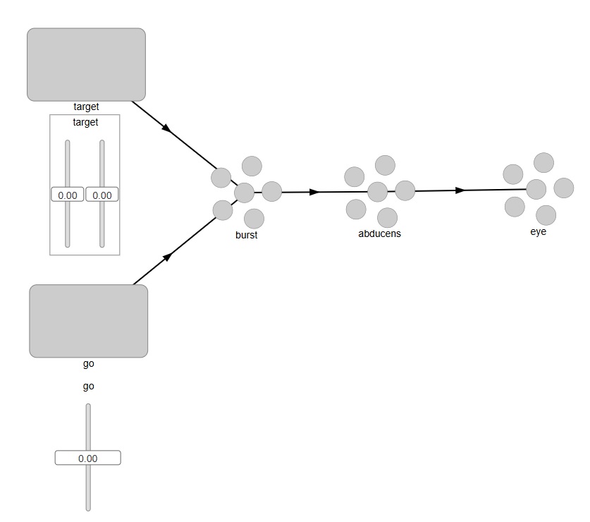
This looks pretty good. In Nengo, external Nodes are squares, and Ensembles are the little circles, so we can intuitively tell what we're looking at. To see inside the objects, we can right click on any of them and bring up details or graphs of activity. However when we actually try to run this we discover that we need two connections from the "go" signal into the burst neurons - one for each axis. Nengo isn't smart enough to connect a single neuron into a 2-d population. (In all fairness, it wasn't designed for that - Nengo's model is more along the lines of "represent and reproduce", which is not exactly what we're trying to do here). What we want is for our "go" signal to gate the movement of the "target" signal through the "burst" neurons. So we have to tell Nengo to perform a multiplication on the incoming target, based on the value of the "go" signal. Furthermore the "go" signal is all or none, so when we move the slider, we only want the gate to open when the slider is at maximum level. The output at the "eye" should be a target position, but only when the gate is open.
Let's see how we would do this in Brian2. With Brian2, we already know we have to let Annie drive. So we will define this simple network inside Annie, as follows:
NETWORK OCULOMOTOR
COORDS(10000,10000,10000)
NUCLEUS EXTERNAL_TARGET
NEURONS 10000
ARRANGEMENT GRID_2
NUCLEUS EXTERNAL_GO
NEURONS 1
NUCLEUS EXTERNAL_EYE
NEURONS 2
ARRANGEMENT GRID_1
NUCLEUS BURST
NEURONS 10000
ARRANGEMENT GRID_2
NUCLEUS ABDUCENS
NEURONS 6000
If we don't give Annie an ARRANGEMENT specification, it will simply organize the required number of neurons in a "pool", that very much resembles a Nengo Ensemble in one dimension. If we don't tell Annie what to do, it'll assume that it's free to do anything it wants - so for our 2-dimensional structure we have to issue explicit instructions. Whereas, the "Go" signal only has one neuron so the geometry doesn't matter. Our eye has 2 eye muscles, one lateral and one medial. We tell Annie GRID_1 so we can distinguish them. The abducens simply becomes a pool of neurons organized in no particular way, except that its inputs will be organized along two one-dimensional gradients, as we're about to see.
Now we can define the connections, as follows:
CONNECTION FROM TARGET TO BURST
TOPOGRAPHY POINT
DIVERGENCE 1
CONNECTION FROM GO TO BURST
DIVERGENCE 10000
TYPE INHIBITORY
CONNECTION FROM BURST TO ABDUCENS
TOPOGRAPHY OMNI
GRADIENT INCREASING
CONNECTION FROM ABDUCENS TO EYE
TOPOGRAPHY GRID_1[0]
With these specifications, Annie will connect the target to the burst neurons in a 1-1 manner in two dimensions (since both nuclei were defined as 2-dimensional). The connection from the single "Go" neuron to the abducens is defined with a divergence equal to the number of neurons, so it will connect with all the abducens neurons. Similarly, the connection from the burst neurons to the abducens is defined as OMNI, so every burst neuron will connect with every abducens neuron. And finally, we're telling Annie to connect the abducens output to the horizontal axis of the eye but only on the lateral side (we arbitrarily define index 0 as the lateral side).
As you can see, the "Go" neuron is defined to be inhibitory, so in this network it will be more like a Pause neuron than a Go neuron. This arrangement makes gating a little easier, because it's "release from inhibition", and actually this is probably closer to the way the biological system works (OPN neurons are tonically active and they only release the eye movement when they stop firing).
All we're trying to do here, is get the eye muscle to contract according to the eccentricity of the target. What we want is, the more the eccentric (the bigger the eye movement), the more muscle fibers get activated and therefore the stronger the contraction. We're telling Annie to provide a single output: a value indicating the level of muscle contraction. There's nothing fancy going on, no synaptic plasticity, no learning. All we're doing is a computation on the target position. We'll not however, that this network is only good for one eye movement. There's nothing that returns the eye back to a resting position. We set it up this way so we can do repeated experiments - because once we get this working, we'll need to adjust the synaptic weights to get the right ratio between eccentricity and muscle contraction.
Next we will export this network from Annie, in Brian2 format. The resulting code is as follows:
(Brian2)
Here, Annie has created some differential equations for us, based on its own internal catalog of available functions. As long as we don't modify these functions inside Brian2, Annie will know what to do with them. Annie will also graph the network for us, so we don't have to depend on Brian2's internal network displays (which are somewhere between inadequate and nonexistent). We want to see the network in geometric form, instead of depending on Brian2's internal neuron "indexes".
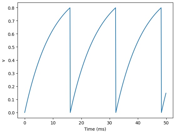
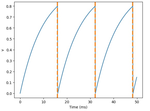
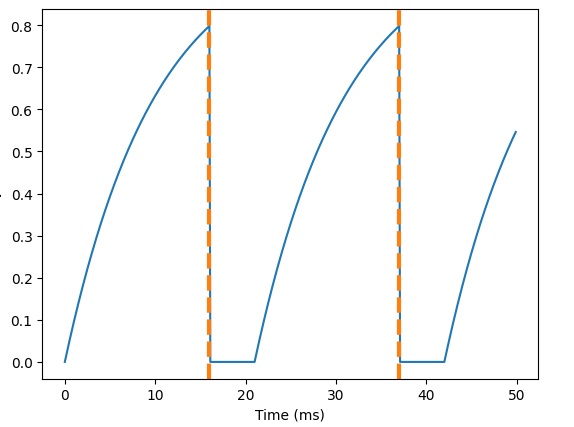
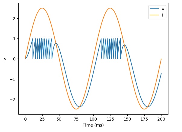
Nevertheless, the network does work, and here are some of the results from a sample run:
(Brian2 results)
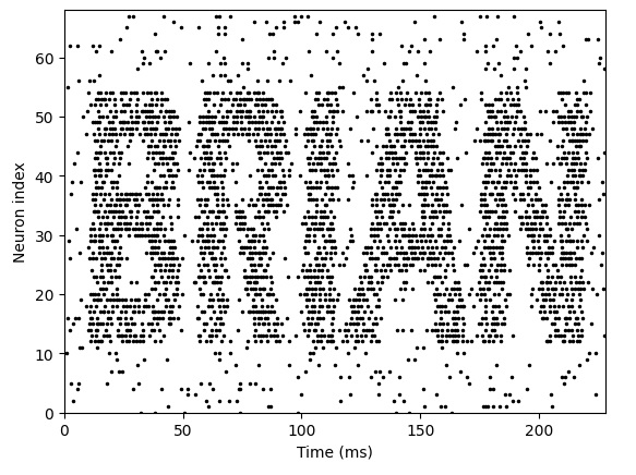
As you can see, Brian2 is doing something quite different from Nengo. To figure out the difference, we need to look at the firing sequences of the neurons, as well as the synaptic activity. Once again, Annie can help us. In both cases (Nengo and Brian2, as well as most other simulators), the firing sequences are available to us after each tick, and Annie can display a hot-cold map for us that intuitively shows us where the activity is.
(Annie hot-cold map)
Here, we run squarely into the issue of geometry. Even when the nucleus we're looking at is non-geometric! What we can clearly see, is that there is no relationship between 2-d geometry and the activity of Nengo neurons. Whereas, the relationship in Brian2, is clear and obvious. The hot-cold output from Nengo is haphazard, there's no obvious relationship between neuron location and amount of activity. Whereas, the hot-cold map from Brian2 shows us that upon stimulation, "all" neurons in the abducens increase their firing levels. This behavior is the direct result of Nengo's internal Ensemble model. It's doing something different under the covers. So we can pick and choose which model is closer to our needs. If we need biological realism, we have to go with Brian2 - but if we just want to control a robot, Nengo is much better for us.
Oculomotor IntegratorAnother interesting and very useful experiment is to model the oculomotor integrator that maintains eye position after a saccade. It turns out in this case, that this behavior is a lot easier to accomplish in Nengo, than it is in Brian2. Unfortunately we can't mix and match simulators, we have to choose one or the other for each experiment.
In the Nengo version, all we need is a single value from the integrator, based on a single value from the abducens. The abducens population will have a certain aggregate activity level, and this will be translated into a single "maintenance value" by the integrator. Therefore in Nengo, the integrator becomes a single Ensemble, and all it has to do is read the input, save it, and map it to the output. Turns out, there is already an existing Nengo model for a Nengo integrator (in fact, more than one! Nengo is a popular simulator). To examine it, we can use the Nengo examples.
with model:
# Connect the population to itself
tau = 0.1
nengo.Connection(
A, A, transform=[[1]], synapse=tau
) # Using a long time constant for stability
# Connect the input
nengo.Connection(
input, A, transform=[[tau]], synapse=tau
) # The same time constant as recurrent to make it more 'ideal'
This is a pleasingly small definition, and apparently the important part is "tau", and the definition of the synapse. In this integrator, the neuron population is excitatory, and it connects to itself. The input is also excitatory. So why don't we get a runaway integrator? The answer is that tau is set to 0.1, which keeps the network behavior stable.
In the Brian2 version, we need to do more things by hand. We have to tell Brian2 to integrate the activities from the 6000 abducens neurons, map them into the integrator, and perform a neuron-to-neuron computation that results in the saving of the level and the transmission of its final value to the output. Therefore we also have to tell Brian2's synapses how to behave.
Already there is an interesting difference between Nengo and Brian2. In Nengo, we just set tau to the value we want.
tau = 0.1
In Brian2, we have to include units.
tau = 20 * ms
Let's see what the rest of a Brian2 network definition looks like:
#
# 100 neurons with refractory period
#
N = 100
tau = 10*ms
v0_max = 3.
duration = 1000*ms
eqs = '''
dv/dt = (v0-v)/tau : 1 (unless refractory)
v0 : 1
'''
G = NeuronGroup(N, eqs, threshold='v>1', reset='v=0', refractory=5*ms, method='exact')
M = SpikeMonitor(G)
G.v0 = 'i*v0_max/(N-1)'
run(duration)
figure(figsize=(12,4))
subplot(121)
plot(M.t/ms, M.i, '.k')
xlabel('Time (ms)')
ylabel('Neuron index')
subplot(122)
plot(G.v0, M.count/duration)
xlabel('v0')
ylabel('Firing rate (sp/s)');
#
# synapses
#
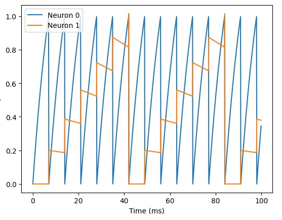
eqs = '''
dv/dt = (I-v)/tau : 1
I : 1
tau : second
'''
G = NeuronGroup(3, eqs, threshold='v>1', reset='v = 0', method='exact')
G.I = [2, 0, 0]
G.tau = [10, 100, 100]*ms
S = Synapses(G, G, 'w : 1', on_pre='v_post += w')
S.connect(i=0, j=[1, 2])
S.w = 'j*0.2'
S.delay = 'j*2*ms'
M = StateMonitor(G, 'v', record=True)
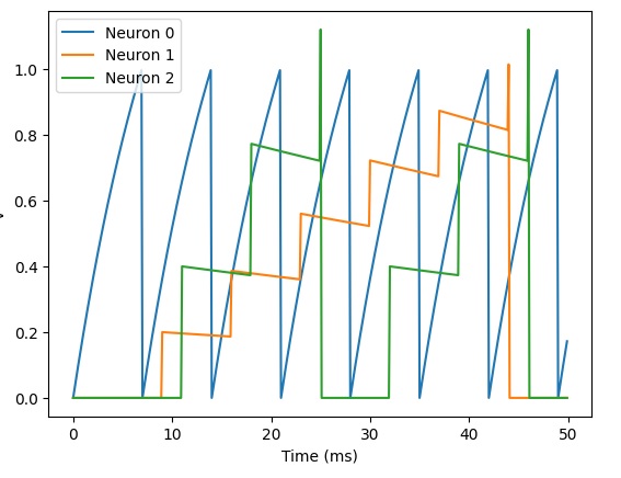
run(50*ms)
plot(M.t/ms, M.v[0], label='Neuron 0')
plot(M.t/ms, M.v[1], label='Neuron 1')
plot(M.t/ms, M.v[2], label='Neuron 2')
xlabel('Time (ms)')
ylabel('v')
legend();
#
# connecting synapses
#
N = 10
G = NeuronGroup(N, 'v:1')
for p in [0.1, 0.5, 1.0]:
S = Synapses(G, G)
S.connect(condition='i!=j', p=p)
visualise_connectivity(S)
suptitle('p = '+str(p));
This code, while logical, is not always intuitive. For example the "for" statement in the last block of code has three arguments that are not entirely obvious. In this particular integrator effort, Nengo is a bit friendlier for us. We encounter this dichotomy a lot, where one simulator is better at something, and another simulator is better at something else. We have to decide though, because we can only use one. So typically we have to explore all the subsystems first, and then make a decision at the level of the whole model. Sometimes, we'll change our minds in mid-stream, because models are typically built incrementally, and at some point we might realize "hey, this isn't working" and choose a different direction. This is unavoidable, it happens a lot and it's part and parcel of the modeling process.
These first couple of experiments weren't too painful, we got pretty good results with a minimum of effort. Now let's see if we can do something more complicated. Let's look at the actual targeting system inside the superior colliculus. Target MappingAt this point we are ready to think about connecting the targeting system at the level of the superior colliculus. The biggest challenge in the peripheral oculomotor system is converting the spatial map in the superior colliculus into the appropriate combination of muscle contractions. This involves deciding when to initiate an eye movement, and it involves calculating the required movement relative to the target position. For this, we need geometry, because there are retinotopic mappings in both the superior colliculus and the cortical areas feeding it.
Next: Memory
|