The visual portion of our model requires a full cortical visual system, for two reasons: first, we need to be able to handle the binocular disparity processing related to depth perception, and second, we need to be able to identify targets for our oculomotor system. However we will begin in the retina, and move centrally. We will first build a retina consisting of four types of photoreceptors, and about 20 types of filtered output channels. These channels will connect into the LGN, where they will interact with thalamo-cortical relay cells. Once in the cortex, the retinal image will be processed for color, motion, disparity, and so on - and all these maps will be topographically aligned. Subsequently, we will follow the pattern in the human brain and build two streams of visual information, one related to object identification and recognition, and one related to object position and movement. They will join in the region around the hippocampus, where they will be phase encoded by a theta rhythm. The purpose of each of these transformations will be exposed and analyzed in detail.

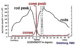
For modeling purposes, we don't need a full visual system. As alread mentioned, we can do a lot with just a small patch of retina and a few moving stimulus templates. If we wanted to get fancy, we could replace the input system with a real camera. This way we can train our network on real life images, rather than contrived templates. There are 100+ million photoreceptors in the retina, but we can reduce this to 10 million with a 4K camera or 1 million with an ordinary 1080p. We don't have to use the entire camera width, we can just use 1024x1024 or whatever convenient dimensions are available to us. There are about 6 million cones in a human retina, and one of the important considerations is to keep the ratios consistent, so for our purposes we could reduce to 1 million cones and thus 20 million rods, and it turns out this is almost right for a 4k camera. If we want to push the envelope there are 100+ megapixel cameras that will give us a full retina, but if we do this we also have to perform all the computations downstream, which slows everything down and doesn't really help us much in terms of demonstrating functionality.

We would also like a camera with an attachable lens. The mounting has to be absolutely correct and secure, and may likely have to be machined. We'll assume we have a machinist available, and we can fabricate and mount the appropriate lens. As a reasonable compromise that still gives us acceptable visual acuity, we can use a full frame sensor in the 24 mPixel range. They are commercially available in convenient forms of packaging.

If we use a camera in this way, the topography is defined for us and all we have to do is assign a coordinate to each neuron. This coordinate will then have to match whatever's in the LGN, and in the SC, to align the retinotopic maps correctly. To allow our retinal output to self-organize onto the LGN topography, we'll define three chemical markers for the LGN, two for retinotopy and one for the layers. We'll do the same thing in the SC.

We don't want to use millions and millions of neurons in our simulator. However some visual acuity is required, and so we have to find a usable intermediate point where we have "enough" acuity for simple tasks without running out of memory or overwhelming the CPU. We're not trying to build an actual robot inside the simulator, we're merely trying to verify that our mathematical logic for building the network is correct, and that the resulting network behaves the way we think it should. Nevertheless, let's continue the discussion on a high-resolution basis for a moment, and then we'll figure out how to back up into something usable.

Topographic Mapping

Our first step is to define the coordinate axes in the retina. In humans this is done on the basis of genetic markers that are exposed in the form of gradients in the developing retina. To stimulate the retina, we can use a camera, and the trouble with cameras is they're flat. The resolution is adequate (a 4k camera screen is about like a retina with 10 million outputs), but the distribution of pixels in a flat camera is not the same as the density of photoreceptors in a round retina.

A human eye is approximately spherical, but slightly flattened at the front and back, forming an oblate spheroid. It's about 24 mm in anterior-to-posterior diameter, with a width of 24.2 mm, height of 23.7 mm, and an axial length between 22 and 24.8 mm. Knowing this mapping, we can construct a linear map between the camera's topography and the retinal topography, and we can build appropriate lenses and simply place them over each camera. Within the eye itself, the retina covers about 65% of the back of the eye, so we can determine exactly how many photoreceptors there should be and where they should be, since we have the density information for humans.

So therefore we will want to curve our retina, and everything in it. We can do this using the method outlined on the previous page, but there are easier ways to do it. If all we need is a curve, we can get that with a simple linear transform. Applying the same transform to all the objects won't change the connectivity, but it will result in a new geometry. The new geometry can then be verified against the declared connectivity, for example if a cell has gone outside the nuclear boundaries it can be identified.

Once we have a visual field mapping, we need to map the pixel outputs from the camera, into hyperpolarizing potentials in our virtual photoreceptors. Before we do this though, we need to think carefully about the mosaic organization of our photoreceptors. They're not like pixels where the RGB values are encoded in a single word. However we can easily separate the R, G, B, and X components (X being a rod, which could be either grey-scale or at wavelength) at each point, and if we keep a local buffer we can also include short-term dynamics. We're going to map the photoreceptors into horizontal cells and bipolar cells. Each of these will draw from a memory array holding the current photoreceptor membrane potential.

We will separate and/or multiplex channels from the very beginning. Our first task is to derive the rod bipolar cell behavior, and that of the 11 types of cone bipolars. To do this we have to arrange the retinal mosaic, then add the horizontal cells and verify the surround, and finally add our bipolar cells with the two different kinds of glutamate receptors. The rod bipolars don't contact ganglion cells directly, instead they contact amacrine cells which then contact the nearest on and off cone ganglion cells. (The rods "usurp" the cone pathways in low light conditions).

One of the interesting features of the retina is the electrical syncytium created by gap junctions between horizontal cells. The horizontal cells create the surrounds for the bipolar cells, which can be up to 25 times bigger than the extent of the dendritic tree, because of the syncytium. The characteristics of the syncytium depend on the kinetics of the connexin proteins forming the gap junctions. We can envision an experiment where we modify the time constants and conductivity to see how these affect the bipolar cell activity. But that's not what we're doing right now, we're just trying to build a retina.

But speaking of electrical activity, the axons of bipolar cells mostly use graded potentials, however the fastest group uses action potentials as well. The bipolar cells stratify in the inner plexiform layer, the fastest cells are in the middle between the on and off substrata. Ganglion cell dendrites ramify in the strat of the inner plexiform layer, and use only action potentials to send signals into the optic nerve. And, to fully account for retinal behavior, we need to include the outputs that belong to the internally photoreceptive ganglion cells, which are used in the maintenance of circadian rhythms and in the reflex related to pupil constriction.

Self organization of the retinotopic map into the LGN can proceed as soon as the ganglion cell mosaic is behaving properly. We'll use the same strategy for the LGN and the SC, a pair of markers and a self-organizing map. We can choose whichever form of SOM works best. The map from the LGN to V1 in the cerebral cortex is a little more interesting. Relay cells synapse in a characteristic manner onto cortical columns, and layer 5 pyramidal cells then project back to the SC, and these maps have to be kept in register. So even though the topography of the cortex is considerably different from that of the LGN, we have to find a way to align the relay neurons with the motor map in the SC.

Network Architecture

At this point we can introduce Nengo, our first candidate simulator. Nengo is a very interesting approach to neural networks, it operates on the Neural Engineering Framework which comes from Chris Eliasmith and colleagues at the University of Waterloo in Canada. This framework uses the diversity of neural properties to create representations of inputs, which it then uses to drive neural action potentials and learn synaptic weights. One of the really great things about Nengo is it's very easy to use. It works on Python code, so some knowledge of programming is required, although they've made it so easy one could do it in one's sleep.

The first thing we want to do is establish the visual pipeline through the cerebral cortex. This is very easy using the Nengo simulator, especially with the Annie interface engine. Annie will output Nengo code, which can then be read directly into Nengo. But to begin with, let's explore Nengo itself, because it's very cool and has lots of great features. Nengo's user interface was written by Terry Stewart, also at the University of Waterloo. We won't get into the user details, you can learn all about Nengo at the Nengo web site.

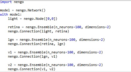
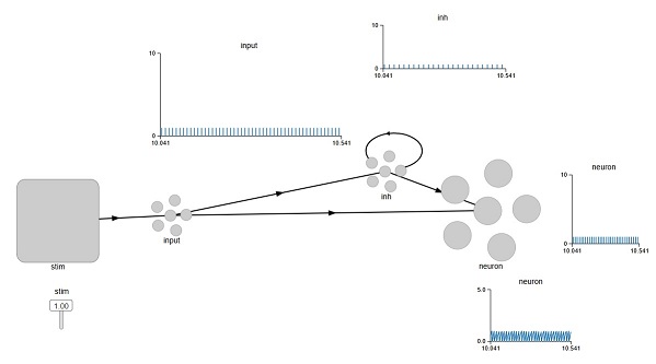
Here is what Nengo looks like. We have defined the early stages of the visual system as a feed-forward pathway. To keep it simple, we have a source of light in two dimensions, so there's only one spot of light and it's only in one position at a time. The network is set up so it "represents" the position of the stimulus. We would like to test the topography to see how well it's being maintained through the various layers.

In Nengo's model, light is a "node", which is different from a neuron. So here, we don't have to create "virtual nuclei" to define things like stimuli and the exit paths of axons. It's nice to see stimuli differentiated from neurons on the screen, Nengo's presentation is intuitive that way. We can verify the topography by moving the two sliders, which represent the X and Y coordinates of the spot of light on the retina. This is the code that generates the network.

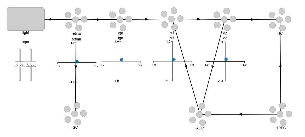
Easy, right? By default, with nothing else specified, Nengo is using leaky integrate-and-fire neurons with a membrane time constant around .01 sec. We can easily change these settings. For now, we're interested in mapping the pathways we'll need to connect into the memory system, the attention system, and the oculomotor system. We can begin by representing the superior colliculus for the oculomotor system, the anterior cingulate cortex for the attention system, and the hippocampus and prefrontal cortex for an episodic memory system.

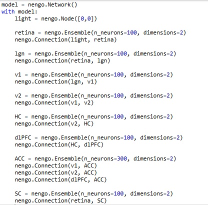
And once again, the code is trivially easy. To begin with, each area has 100 neurons, and this will change as we build the network. We won't need a lot of neurons just to verify functionality, we can easily use a 10x10 retina during testing, which will give us 100 of each type of ganglion cell, and that's more than enough to demonstrate the functionality of a small patch of retina. Subsequently we'll need to abstract some of the information because of the sheer volume, and we'll look at how to compress the volume of information using sparse representation and dimensional reduction and other methods.

Now... there's a little something missing here. We can't see into the retina. We don't know what Nengo's actually doing under the covers. And, there's no actual topography, we're just giving Nengo two coordinates (two "values") and asking it to represent them. An important realization comes when we display the spiking activity of the neurons (we can do this by simply right-clicking on an Ensemble and selecting "Spike Activity"). It turns out, there is no relationship whatsoever between the position or index of a neuron, and its location in the retina. In fact, the simple ensembles we generated have no topography whatsoever! When we look at the spike trains as we're moving the sliders, there's no logical relationship between the behavior of any particular neuron, and the location of the light stimulus. And that is because, the neurons in each ensemble are "encoding" the stimulus values in a manner that is quite unknown to us, and depends on the random slopes and intercepts of neuronal current-frequency curves. Unfortunately, this is enough to give most scientists a bad case of the Willies... but the good news is, it can be easily corrected! The bad news about the good news is, it takes lots and lots of Python code. Here is an example using a single neuron:

import nengo
model = nengo.Network()
with model:
      neuron = nengo.Ensemble(n_neurons=1, dimensions=1)
      # Set intercept to 0.5
      neuron.intercepts = nengo.dists.Uniform(-0.5, -0.5)
      # Set the maximum firing rate of the neuron to 100hz
      neuron.max_rates = nengo.dists.Uniform(100, 100)
      # Sets the neurons firing rate to increase for positive input
      neuron.encoders = [[1]]

      stim = nengo.Node(0)

      # Connect the input signal to the neuron
      nengo.Connection(stim, neuron)

What we have basically done here, is disconnect all of Nengo's wonderful representation machinery, and asked it to simply encode our stimulus value into a single neuron. In doing so, we lose the precision derived from the ensemble, and instead we have a noisy neuron that sometimes skips a beat. (In other words, we have a "real" neuron!). If we want our neuron to be inhibitory, we can modify a connection as follows:

nengo.Connection(c, b.neurons, transform=[[-2.5]])

The transform multiplies the input by a negative number, ensuring that the neuron responds in the opposite way. An interesting thing happens though, when we try to do a self-inhibitory recurrent connection. Look at the graph labeled "inh", that shows the spiking activity of the inhibitory neuron. The stimulus is at maximum, so we expect a very strong drive into the inhibitory neuron, therefore a very strong inhibition of self. But the neuron is still spiking. Why is that?

We can play with the strength of the connection, but it turns out it doesn't make much of a difference. So what's actually going on here? To find out, we'd have to get into the guts of the Nengo simulator itself. If we look at the properties of the Ensemble we see a line that says:

eval_points: ScatteredHypersphere()

What does that mean? Well, at this point we have to look at the Neural Engineering Framework to find out. And we won't get into it, but the point is Nengo isn't quite as easy as it looks. To use it for real science, you have to know quite a bit about it. You have to know how the simulation engine actually works, and what those eval points really are. Which is not something most neuroscientists will know off the top of their heads.

The biggest drawback of Nengo is it's completely unaware of geometry. Fortunately the Annie interface tool will take of at least a part of that, however the Nengo simulator itself will not (currently) use neural geometry to perform calculations, it works exclusively on the basis of the connections and the properties of the neurons and synapses. It's an excellent simulation engine, definitely one of the fastest and most efficient, but it's somewhat limited without the geometry.

In the next section we'll look at another tool, that goes in a different direction. Brian2 is also a very popular simulator, and for some neuroscientists, it can be more intuitive. Brian2 actually lets you write differential equations. You can completely determine the behavior of all your membranes. (In context, of course). Some neuroscientists think like that, they think in terms of differential equations. Not many, though. Very few neuroscientists could recite the Hodgkin-Huxley equations off the top of their heads. Instead, they just want to tell the simulator "this one is a Hodgkin-Huxley neuron", and this other one is a leaky-integrate-and-fire, and so on. Is this enough? Or does one actually have to write differential equations and specify all the time constants? Let's take a look at how Brian2 handles this.