When investigating the brain, models are very helpful. They allow us to explore neural behaviors without sacrificing animals or invading their nervous systems. We would like to understand how behaviors can be precisely timed after just one example. For instance if you're a child learning to play basketball, and someone shows you how to shoot the hoop, you can probably do it all by yourself after one or two attempts.
One-shot learning is an interesting study, but let's set that aside for a moment and look at some model neurons that will help us simplify our investigations. Which model neuron we use, depends on the behaviors we'd like to look at. If we're just interested in the algebra and statistics, we can use simple model neurons that are amenable to matrix multiplication with nVidia GPU's. On the other hand there are many applications for which static algebra is inadequate, and particular kinds of dynamics are required. In order to support both, the neuron must have certain key capabilities, and these are what modeling helps us understand.
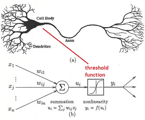
Early Model NeuronsModeling of neurons for computational purposes began with McCulloch & Pitts in 1942. They considered a binary neuron whose state could be either firing, or not firing. The neuron integrates its inputs (as a weighted sum), and if the result is over the threshold the neuron fires, and if it's under the threshold it doesn't. The original threshold function was the Heaviside step function, which is not smooth and can not be easily differentiated. And binary neurons are limited in what they can represent. The ideas embodied in the McCulloch-Pitts neuron later became the basis for an early learning machine called the Perceptron (Rosenblatt 1958). In the Perceptron, the synaptic weights are adjusted based on an error that is determined from the data. The Perceptron essentially "fits" its input to a set of linear parameters. Unlike the McCulloch-Pitts neuron, the Perceptrons use neurons with a sigmoidal threshold function (Rosenblatt 1961), which is differentiable and therefore errors can be passed backward through the network and assigned to their sources in proportion to their contributions.
Simple neurons like these have significant limitations, and based on what we've already seen they're inadequate to mimic biological behavior. Nevertheless they still have useful computational abilities when they're wired into populations. The Perceptron is able to perform "linear separability"on a dataset, meaning it finds the slope and intercept of a straight line that partitions the data. More neurons simply means more lines, the end result is a combination of linear partitions. Linear regression is probably the single most common activity in all of statistics, so this capability is useful. However it doesn't work on all datasets, and the Perceptron is a bit of a one-trick pony in terms of its neural behavior. Unfortunately Frank Rosenblatt passed away before he could counter Marvin Minsky's points about the Perceptron's limitations, but before he died he saw his invention being used in real time national security applications. Even binary neurons can be very powerful when wired into populations and given the right kinds of plasticity.
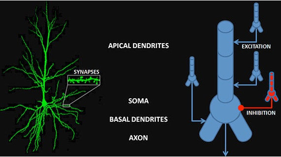
After the successful demonstration of the Perceptron, neuroscientists pointed out that the firing of neurons often uses a "rate code", where the rate of firing is determined by stimulus intensity. The "spike rate" was thought to be a neuron's only output, therefore any information carried out of the neuron must be encoded in the spike train. And so the binary neuron became a linear neuron, where the output can take on any positive value (or zero). In this case the calculation of the threshold still applies, and if the output is above threshold the thresold level is simply subtracted from the output to obtain the final value (this is the principle used in the ReLU function in machine learning). Such a model neuron is shown in the figure, and you can see the only thing that differs is the threshold function.
In the above figure the inputs I are multiplied by the synaptic weights W and integrated over the dendritic surface to arrive at a sum S, which is added to a "bias" term b representing noise or a baseline activity level. The difference between this neuron and the McCulloch-Pitts neuron is that the threshold function f is differentiable. If f is linear like a Relu or sigmoidal (S-shaped) instead of being a step, it can be differentiated, and an error occurring at the output O can be passed back through the threshold and the contributions of each input to the error can be determined. Then, the synaptic weights can be updated to reflect the new error information. The process of passing the error in the opposite direction through the threshold function is called "back propagation".
In some machine architectures, when the derivatives for successive layers can be calculated, the errors can be passed all the way back through the layers in one computational sweep. But brains don't work this way! To pass back an error, it has to be explicitly represented. And models like this are far from Hodgkin-Huxley, in that they contain no dynamics. (For example they don't account for the refractory period). Hodgkin and Huxley are at the opposite end of the simple model neurons whose outputs can be computed in a reasonable time frame. A full GHK model of a biological neuron would involve the numerical solution of half a dozen simultaneous differential equations, which would rapidly become exasperating with networks containing a few thousand neurons. In the 70's and 80's, in an effort to make model neurons more realistic, the essential behaviors of biological neurons were crystallized in several ways.
Simplifying the Hodgkin-Huxley ModelReal neurons have more than two parts, more than just an integrative portion and a spike generating portion. The properties of a neural membrane vary according to its location, for example calcium channels are present in the dendritic tufts of cortical pyramidal cells, and in the basal dendrites, but not in the shafts of the apical dendrites. In general ion channels are carefully localized along the neural membrane, and this is true everywhere, not just in the synapses.
On the other hand, the full Hodgkin-Huxley model for multiple channel types is computationally intensive. There exist simulators for individual neurons (like NEURON and Brian2), and simulators for networks (like TensorFlow and PyTorch), but there's very little in between - and that is because, the behaviors that we require from the neurons and synapses is computationally expensive. With the current state of the art in neural modeling, if someone discovers an exciting new behavior related to calcium channels in a cortical stellate cell, it's quite difficult to subsequently create a network full of such cells and test them under changing input conditions.
While the above simple neurons distill the basics of dendritic summation and a non-linear threshold for action potential generation, they're too simple to handle the complexities of multiple ionic conductances. On the other hand, the Hodgkin-Huxley model is four-dimensional and a little too expensive computationally. Perhaps we can find something in the middle, something a little more realistic that's still amenable to computation. It turns out we have a variety of choices, and a scale of complexity.
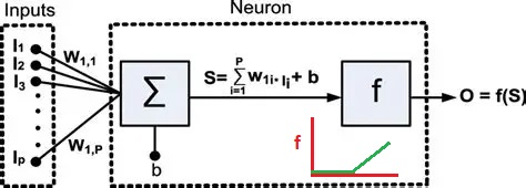
Morris-Lecar ModelOne of the variations of Hodgkin-Huxley students should be familiar with (because it's widely cited and widely used) is the Morris-Lecar model. This is a somewhat simplified version of H-H that still shows bifurcations and spiking activity.
(figure from Rowat & Greenwood 2014)
The drawback of the Morris-Lecar model is it only uses two conductances (calcium and potassium), and it has some significant computational artifacts, both at high frequencies and at certain particular frequencies.
Fitzhugh-Nagumo ModelAnother model neuron that's frequently found in the literature is the Fitzhugh-Nagumo approximation. This model is an abstraction, rather than directly modeling ion channels. It does not display any bursting behavior, nor can it model subthreshold dynamics.
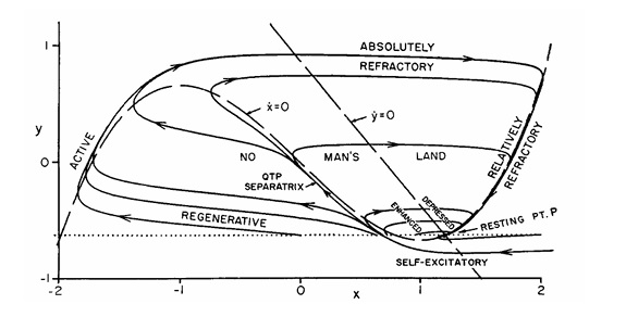
(figure from Nagumo et al 1962)
These model neurons can be useful if we're just trying to replicate simple spiking behavior. However the simplified dynamics can create computational artifacts. We would like a neuron that is computationally friendly and biologically accurate, and that can be modified at least to a limited extent, so we can test the effect of various conductances and various geometries.
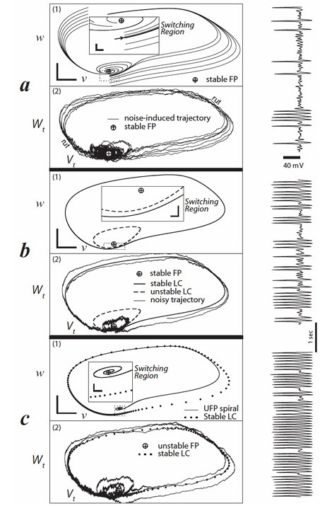
Integrate-and-Fire (Izhikevich) ModelSpike times can be precisely modeled by integrate-and-fire neurons, which are frequently used when modeling TTFS and STDP (please refer to the glossary for the definitions of these terms). Unfortunately this model can create spike trains with arbitrarily high firing frequencies, so one must be careful. There are modifications to the integrate-and-fire model that allow for setting maximum firing rates (Strack et al 2023). The "leaky" integrate-and-fire variant has become a staple in "nearly biological networks". The Izhikevich neurons offer a range of integrate-and-fire behavior that is qualitatively accurate as long as one is not too concerned with the geometry. Geometric specificity gets expensive after a few compartments (and see below for more information on branching and compartments).
(figure from Izhikevich 2003)
A MATLAB tutorial for Izhikevich neurons is given here.
Poisson ModelsThere are some models that are "in between" rate codes and spike times, for example they may use a Poisson approximation to estimate spike times from a rate. Such models are frequently used in oscillator paradigms to conveniently visualize the system attractors. Poisson models are related to gamma distributions, which in turn are related to Bayesian statistics, and gamma functions (which are the integrals of gamma distributions) are related to the fractional calculus which describes past, present, and future events.
A Poisson process can be used to model the interval between spikes. Unlike a Gaussian distribution which is parametrized by its mean and variance, a Poisson process has only a single parameter which is its rate. (The variance of the rate is always equal to its mean). A Poisson process assumes stationarity, that is, the rate does not vary with time. This is of limited value in modeling biological neurons, since real neurons are not stationary. Nevertheless, a Poisson model can create some realistic looking spike trains.
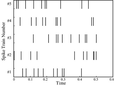
(figure from Amin 2006)
To adjust the ratio of variance to mean in a Poisson model, the Fano factor can be used. If we're looking at a time series and digesting data as it arrives, the Fano factor can vary with time.
Generally F(t) = σ2t / μt
If the Fano factor varies with time, the counting process is no longer a renewal process and a Markov renewal process is needed instead, where transitions are described probabilistically.
To model changes in the firing rate over time, we can use an inhomogeneous Poisson process, which is a stochastic process where the rate varies over time as λ(t). Such a process still assumes independent increments, that is, the number of events in non-overlapping time intervals are independent. And again, this may not be a good assumption for biological neurons, however it has worked in some cases and its relationship to adaptation is noteworthy (Farqui et al 2013).
Poisson-"like" processes are useful in other ways too. Gamma and beta distributions can be used to synthesize Poisson-"like" distributions and the advantage of using these models is the distributions form conjugate priors for Bayesian inference. So, if a synapse or neuron can be related to such a distribution, and the behavior is adjustable based on the data, then the network can be used for things like estimation of likelihood, optimization, and creativity in the generative sense.
Stochastic ModelsThere is a class of models that doesn't depend on the underlying physics and only looks at behavior (these models could be classified as "statistical", or "phenomenological"). The statistical approach uses the inter-spike interval (ISI) as the foundation of its method, and thus is often associated with Poisson dynamics. The subsequent analysis is very much along the lines of data science (using principal component analysis and similar techniques). The advantage of this method is that synaptic modification can be performed on the basis of temporal correlation alone, regardless of the underlying physical mechanisms. This approach has its roots in machine learning, it goes all the way back to Kohonen, Widrow, Hebb, and beyond.
At a more precise level, neurons can be modeled as stochastic generators. This is essentially a better version of the Poisson approach, insofar as the setpoints control the resulting outcomes. The generators can be kept simple, and in a stochastic system the Wiener process is about as simple as it gets. Unfortunately the assumption of stationarity is violated in many ways in biological systems, and the real situation is closer to nonlinear non-equilibrium thermodynamics.
Stochastic modeling, is where the math gets complex. To understand neurons in their full stochastic glory, an engineering education is necessary. This is because the resulting relationships invoke a class of physical models that includes the Langevin formalism, Fokker-Planck equations, the Ornstein-Uhlenbeck process, and stability considerations such as Lyapunov exponents and Routh-Hurwitz criteria. However stochastic modeling is vitally important for research in neuroscience, because it helps us understand behavior in the phase plane, including oscillations and the transitions between states (notably bifurcations, especially Hopf bifurcations). Stochastic modeling is as close to ground truth as we presently come, in terms of biological realism. When combined with information geometry, stochastic neurons support powerful and realistic network models.
Stochastic modeling is also directly applicable to the growth of a neural network, for instance the ability of axons to find their targets, and the pruning that occurs on the basis of incoming stimuli. Stochastic modeling is important at the molecular level too, to understand the release of synaptic vesicles, the binding of neurotransmitters to receptor sites, and the mechanical coupling associated with active transport and the management of receptor concentrations.
Stochastic models are, unfortunately, computationally intensive. One of the primary drivers of computation time is the need to generate random numbers. More often than not, the random numbers need to be drawn from a distribution, so methods like the Metropolis-Hastings algorithm are invoked, and these can become inefficient when the distributions get tight. The primary issue is one of scale. Realistic network simulations require millions of neurons, and in today's world the only alternative to supercomputers is arrays of neuromorphic FPGAs. If there is a device that mimics a neuron, it must be small and it must consume a tiny amount of energy, because many of them would be required for an entire network. Lately there are photonic devices that can generate true random numbers at rates in the gHz range, which is very helpful for fully asynchronous processing. Even so, a single cortical neuron may receive 10,000 synaptic inputs, each of which is plastic according to a set of a dozen or more molecular kinetics. This is plenty to keep a powerful simulator busy.
The amount of stochasticity and "noise" can become an important factor in networks operating near criticality. Some randomness is useful, for things like escaping from local minima in an optimization scenario. But correlated noise disrupts communications, especially in topographic networks (which is "most of them", in a human brain). The amount of noise can affect network dynamics, and it can also affect things like the separability of data and representations. There are many ways to "de-noise" a set of inputs, we'll look at some of them in the section on wavelets.
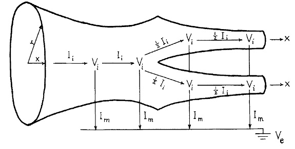
Connor-Stevens ModelJust for completeness, if there's a supercomputer available we can go the other way, and make our neurons as biologically precise as possible. An example is the Connor-Stevens model, which includes a transient A-type potassium current that enables more complex firing patterns like spike frequency adaptation and delayed firing. For our purposes, one of the more enlightening aspects of the Connor-Stevens model is its exposure of the current-frequency curve of neurons. An example is shown in the figure.
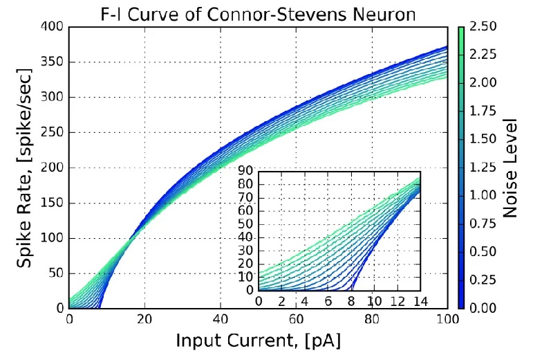
Assuming this curve is measured near the axon hillock where the action potential is generated, the current is the summed current generated by all the synapses along the nerve membrane. In biological systems this curve typically has a wide range, induced by the variation in the distribution of channels in individual neurons. We can use this variability, to a limited extent, to encode information along a single dimension. This method is available in the Nengo simulator, which we'll survey in the section on modeling.
There are some excellent videos on YouTube that discuss neuronal dynamics in more detail, for example the series by user neuronaldynamics5989.
CompartmentationIn addition to the timing of action potentials, there are also questions relating to the integration of signals (data) along the dendrites. Among them are the issue of membrane multi-stability, the issue of dendritic spiking, and the issue of sub-threshold membrane oscillations. The latter issue can affect both integration and spike generation, and possibly serve as a control point for one or both.
One of the key features of neurons is that their processes branch, and sometimes the branching geometry can be very different from one end of the neuron to the other. Dendrites in particular are geometrically important because of their surface integrative properties, and even within the same neuron they can have different lengths and diameters, and different concentrations of ion channels that are compartmentalized and kept in place by the cytoskeleton.
The classic compartmental model for dendrites is still the Rall model. In this model, dendrites are treated as passive cable conductors. (The model was created before the discovery of spiking dendrites). Dendrites are modeled as branching trees of equivalent cylinders (an extension allows for tapering).
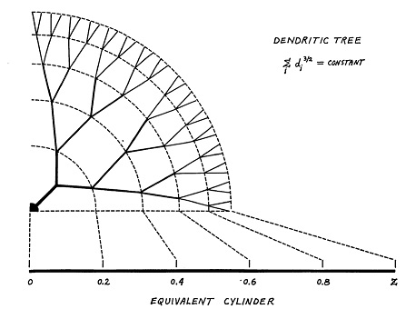
(figure from Wilfrid Rall - CC BY-SA 2.5)
(figure from Wilfrid Rall - CC BY-SA 2.5)
Within a dendrite, compartmentation is further enabled by the architecture related to spiny synapses. The thin stalks of dendritic spines help to restrict biochemical diffusion, essentially creating an independent compartment in each synapse. The communication out of such compartments is often complex, involving multiple stable states in the nearby dendritic membrane. In addition to ordinary graded potentials and plateau potentials, spiny synapses can generate dendritic mini-spikes that travel into the cell body, where they may convert the neuron from from one state to another.
Spiny synapses are vitally important to understand computationally, not only because they're ubiquitous, but because the integration of dendritic mini-spikes can occur quite differently from the passive forms of integration usually promoted in the classroom. In the simplest case, mini-spikes are generated by two or more successive excitatory inputs (within a very narrow window, say a few msec). The propagation of mini-spikes can fail at branch points, however when it succeeds the propagation of mini-spikes into the soma can force the neuron into a high-throughput "up" state, where subsequent inputs can affect bursting. At the moment the regulation of this process is poorly understood, and it is an area of active research. It certainly involves at least two different kinds of glutamate receptors, calcium, proteins like CaMkII, glial cells, transcription factors, and the spine apparatus and its endoplasmic reticulum. The activation of "hot spots" in the data and their translation into "up states" in neurons is one way in which criticality can be controlled at the modular level in the network.
Sculpting Population BehaviorAt the end of the day, the behavior of a neuron is determined mainly by its ion channels. These channels can have different kinetics, they can be voltage sensitive or not, and they can have different conditions for activation and deactivation. One can model such behaviors using programs like NEURON or Brian2, but they're very difficult to implement in machine learning situations with TensorFlow or PyTorch, because the latter specialize in matrix multiplication and can't really handle dynamics. So the machine learning community encodes the dynamic in various ways to approximate the desired results. We are just now at the point where the neuroscience and machine learning communities are beginning to inform each other. I started modeling neural networks in 1978, long before they were a thing - and there was no one in the field at that time, only a handful of forward looking researchers who were often perceived as eccentric bordering on crazy. I was at Princeton when John Hopfield wrote his Nobel prize winning papers, and at the time no one took notice, they were considered an interesting oddity in the physics community. (But I noticed - I was fresh off extracting Volterra kernels from the lateral line organs of sharks and skates, and I looked at Hopfield's first 1982 paper and started laughing. "Binary neurons!" I said, and put the journal down. The next day I was back in the library looking at it again, because something about it caught my attention). And then it was a few years before Hinton and Sejnowski and David Tank and others expanded Hopfield's models and invented the Boltzmann machine (and demonstrated NetTalk - the video is still on YouTube).
The building blocks for neural populations are just like the building blocks for electric circuits. There are components, and there are wires. In biology as in electronics there are hundreds of different kinds of components, but unlike in electronics, biology has different kinds of wires too. Some of the biological wires behave in highly nonlinear ways, and they enable some special-purpose behaviors which would otherwise be nearly impossible to accomplish by traditional means.
The computational power of neurons is in populations. Neurons by themselves do very little, but when they're hooked together they become very powerful. And, when engaging in the modeling of neural populations, it helps to have an interactive environment with a friendly GUI and a powerful computational engine. Such environments are available, usually for free for individual and student use. For example Nengo is a wonderful interactive modeling environment, and it interfaces with all manner of computational engines, even neuromorphic hardware. Using such an "IDE" makes turnaround times much faster. We'll see some Nengo output when we begin modeling in a few short pages, and there are many useful simulation environments, including NEURON, Brian2, and Nest. We'll look at them all.
Next: Neurons in Populations |