So far we've talked about neurons and synapses, and we've seen one example each of a sensory and motor system. Relative to a sensorimotor timeline, we have the picture of a linear sequence of layers of neurons, and we also have the picture of a topographic mosaic involving processing modules having connectivity both within the layer and from layer to layer. We have not yet discussed compactification, or topological embeddings. But we can begin to do so, and in the process start tying together some of the diverse viewpoints we've encountered so far. A good place to start is by looking at the underlying mechanisms of synaptic plasticity, as they relate to data-driven self-organization.
At this point we should keep in mind that the purpose of the brain is to optimize the behavior of the organism in real time, and that the brain is a computational window moving through physical time for exactly this purpose. In doing so it obeys physical laws, but it is nonlinear, and it has memory, and it often operates far from equilibrium, meaning that we can not adequately model it with simple linear systems. We know this in advance, so the simple models on this page are meant to illustrate simple principles. The first and most important is the idea of real time optimization, which in our case means "precision around T=0".
Timeline OrganizationLet's begin by organizing some of the systems we already talked about, into a neural timeline centered on "now". We talked about the visual system, and how the retina sends it information, and we talked about the oculomotor system, and how it brings targets to the fovea. The point of control between these two systems is out in space somewhere, that is to say, the eyes focus on a point in visual space, and then the information from that point is fed into the brain. How does the brain know, whether the point in focus, is actually the point that was desired?
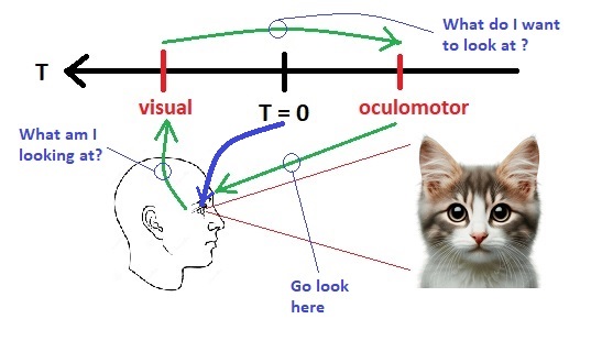
Fixation is a rather complex reflex, as it involves the acquisition of an object whose coordinates have been determined relative to the current eye position. Therefore, the visual image must be processed first, the boundaries of objects detected and stored, the objects identified (or at least indexed) for target selection, and then the target information encoded and transmitted to the oculomotor system. Machines can do this, but they require sophisticated programming. Human beings self organize, the connections form all by themselves under very limited genetic guidance, and the biggest part of self-organization is the neural system coming to represent the properties of the data itself. The organism can best align its movements with a changing environment by learning the properties of the environment and adapting to them. Such adaptation happens in both space and time, since the fundamental piece of input is a moving stimulus.
Sources of VariabilityThe simplest and best studied aspect of neural self organization is synaptic plasticity. In real life this gets increasingly complex, with dozens of neurotransmitters and receptor types regulating themselves and their neighbors - but we can easily illustrate some basic behaviors with simple computational models. Historically one of the most important concepts that developed around the turn of the 20th century is that neurons that fire together somehow strengthen their mutual connectivity. This idea was formalized by the psychologist Donald Hebb in 1949, in the form of a temporal correlation window between the firing of a neuron and the synaptic activity that immediately precedes it. In a discrete time setting the equation might look something like:
dW(i,j) = W(i,j) + α A(i) A(j)
where α is a learning rate and A(i) is the activity of neuron i. When both neuron i and neuron j are above threshold at the same time, the strength of the synapse from i to j is increased by a factor α. We can get the synaptic strength to decrease instead, by making one of the neurons inhibitory or by changing the sign of α. In real neurons the time course of synaptic events is variable and usually represented as a combination of exponential rise and decay, like this:
v(t) = H(t) * (e -t/τ)
where H is the Heaviside step function and τ is the decay rate. If we need a smoother shape we can multiply the decay by t so it rises nicely before decaying.
v(t) = H(t) * (e -t/τ) * (t / τ)
An even broader library can be achieved by combining exponentials.
v(t) = H(t) * (e -t/τ - e -t/τx)
with τ != τx so the rise and fall times are kept separate. This approach nicely shapes the PSP and allows for a wide variety of time constants. These two parameters are often sufficient to represent complex behavior. The figure shows some of the PSP (post-synaptic potential) shapes that can be acheived by combining exponentials.
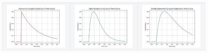
(figure from Brian2 simulator documentation)
The shapes of post-synaptic potentials are a source of variability in networks. Even with strict genetic programming, each synapse is ever-so-slightly different. Computationally, this means we have to solve an ordinary linear time invariant differential equation with constant coefficients for each synapse at every time step. That's a lot of equations, but it can easily be handled by a laptop CPU with a reasonable amount of memory.
Another source of variability arises in the neurons themselves, in the form of variations in the slopes and intercepts of current-frequency curves.
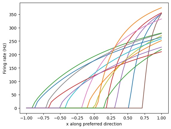
(figure from Nengo simulator documentation)
Here the "preferred direction" is simply a representation of the input current, it's approximately G * (V-Vr) where G is the conductance and r is the resting potential. These curves can be positioned and clustered, and their slopes and intercepts adjusted to create a range of desired responses. To derive this information from a real biological system, multi-electrode stimulation and recording or repeated single-electrode penetration would be needed. Such curves can not easily be derived from tracer imaging or calcium imaging, however they can be easily investigated with a computer model.
Again, the value being represented is simply the total input, that is to say the sum of the post-synaptic ionic currents affecting the neuron membrane. The I-ν mechanism is helpful when encoding a single value, because neurons can support this behavior in the absence of synaptic modifications. Together, these forms of variability represent a powerful combination. It is unclear whether the neuron parameters can learn and modify themselves like the synapses can. The most likely answer is "probably not", although somatic behaviors can definitely be influenced by other mechanisms that "can" learn. A more likely form of learning in this case is indirect, for example through modulatory synapses that temporarily change the response properties. The current-frequency curves are directly related to the time constants and positioning of ionic channels in the neuron membrane, and can therefore be modulated. When channels turn on and off, these curves can change.
The more common and better known form of variability is the synaptic "weight" discussed above. In this case, weight simply means strength. One could consider it in terms of the ratio of post-synaptic effect to pre-synaptic driving signal. As discussed in the earlier section on synapses, synaptic transmission is vesicular and quantized. This behavior is rarely detailed in simulations, except when we need to study vesicular depletion related to calcium levels, and other such low-level behavior (which may enter into the picture, for example, when studying synaptic depression). Instead, the synapse is simply assigned a "strength", or weight, and equations are formulated to change the weight over time. Such equations are called "learning rules".
There are many forms of learning rules. The classic Hebbian behavior is usually associated with some combination of STP/STD and LTP/LTD, and modeled by a simple equation of the form shown above.
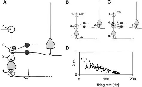
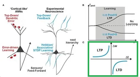
An example of a more sophisticated learning rule is spike timing dependent plasticity (STDP), which combines LTP and LTD in opposing manners to get bidirectional behavior around T=0.
In practice, we'd like to make sure that the learning algorithm actually converges, and a common way of doing this is to adjust the amount of lateral inhibitory influence in the network. Topography can be conveniently specified in terms of convergences and divergences along the principal geometric axes. Whereas the retina is topographic (and so is the cortex and the oculomotor targeting system), the oculomotor integrator is not, and at some point there must be a translation between the two-dimensional visual topography and the one-dimensional code that determines eye muscle contraction. In humans this translation is accomplished by a combination of "encoding" in the manner shown earlier for the Seung model, and gradients of connectivity from the targeting system to the burst neurons.
We can note at this point that the synapse-related behavior of individual neurons can be adjusted in more ways than just by altering the weights. For instance there is an interplay between the position of synapses along an elongated dendrite, and the distribution of ion channels. An example is the layer 5 pyramidal cells in rat cerebral cortex, which have a gradient of an Ih conductance that increases linearly with distance from the soma (Williams and Stuart 2000). This tends to counteract the effect of distance-related passive cable losses, effectively bringing synapses at varying distances closer to each other. The point is that geometry is important, and the behavior of ion channels often plays directly into the population behavior at the network level.
Another important axis of synaptic variability is the precision of spike timing between neurons. The time constants associated with conductances in excitatory and inhibitory neurons may vary widely. For example in the CA1 field of the hippocampus, the kinetics associated with inhibitory neurons are very fast, while those associated with pyramidal cells are slower (Fricker and Miles 2000). This is a meaningful exploration of one of the simple connection motifs shown earlier in relation to the LGN, but in this case the same motif is present in the hippocampus.
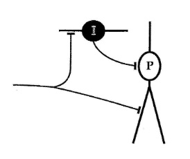
In the hippocampus, pyramidal dendrites generate plateau potentials in the absence of inhibition, that tend to prolong the incoming EPSP's. But when the fast inhibitory neuron is activated, the plateau potential disappear and the pyramidal neurons do not generate late spikes. These are all examples that contribute to the self-organization of neural networks, and in many cases complex behaviors can be derived from simple building blocks. Timing is important. The timing of synaptic modification occurs "relative to" the action potentials generated by neurons, thus the synapse has to respond within the millisecond or two that contains both the action potential and the synaptic potential. The tau associated with the synapse should be in the same range as the tau associated with the action potential. Even if the learning rule has an exceedingly long time constant, it must still be timed in relation to the original action potential that triggered it. Some good resources for understanding the time constants related to synaptic behavior are here and here.
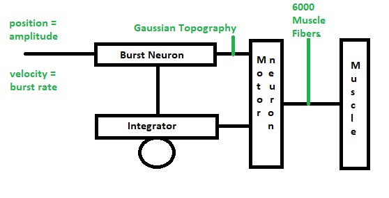
Elementary Self-OrganizationAs an elementary example of self-organization, it's helpful to consider the oculomotor integrator. It takes a burst input from an EBN neuron, and converts it into a value representing eccentricity (target position), which it holds, and forwards to the motor neuron. The incoming code is a burst rate, the amplitude of the saccade is linearly related to the firing rate within the burst. We need to control three things precisely: the beginning and ending of the saccade, the amplitude of the saccade, and the acquisition of the target as determined by an error between target position and the visual axis of the fovea. From a control systems standpoint, this translates into a set point and a gain, along with some start/stop logic. The gain is to be set "such that" the target is as close as possible to the fovea, after the eye movement.
Since we are focusing on the oculomotor integrator, we will assume that the topography of the visual and motor maps has already been aligned for us (during earlier development, as it were). We will focus solely on the synaptic plasticity ("learning") that has to occur to set the oculomotor integrator gain and time constant. We'll begin with the simple case, which is movement in only one dimension, corresponding to the horizontal axis controlled by the adbucens motoneurons. Later we'll have to consider the possibility of a joint integrator representing both (or all three) axes, especially since there seems to be such an integrator related to the medial vestibular nucleus, which is directly connected into the oculomotor system.
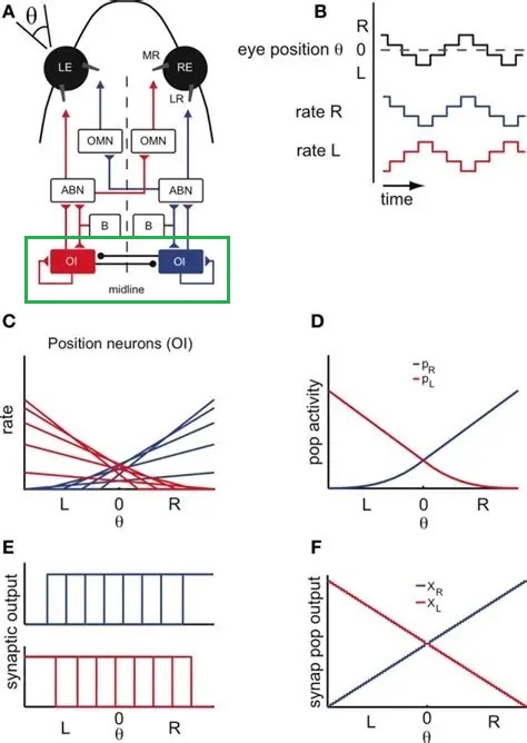
The figure shows the anatomical arrangement of the integrator. It also shows a possible source of variability in the relationship of eye positions to neuronal integrator response curves. In this integrator, we're interested in the connections from the integrator to the abducens motor neurons, and the connections from integrator neurons to themselves. The latter have to be just strong enough to maintain eye position after the burst neuron has disengaged. From biology we know that the integrator has a time constant of around 25 seconds, and that it is leaky. The amount of leak has to balance the amount of self-excitation. In this schematic there is no pause neuron, but we can include one if we wish, to reset the integrator (and therefore the eye position).
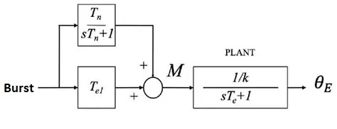
We can represent the desired arrangement from a control system standpoint, as shown in the figure below. Here M is the abducens motoneuron, and the recurrent excitatory connection in the integrator population has been incorporated into the transfer function.
A similar control system occurs in the VOR reflex, between the vestibular system and the oculomotor system. The VOR integrator converts head velocity to eye position. The three control system versions in the figure below are mathematically identical in the transfer space, but exhibit a different range of boundary dynamics. In (b), the recurrent excitatory connection is shown explicitly and forms an essential part of the integrator. Note that it's a recurrent feedback connection rather than the feed-forward connection shown above.
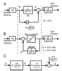
(figure from Chan & Galiana 2005)
Integrators like this are ubiquitous in the peripheral nervous system, and they all likely use similar mechanismss. Variability in representation is achieved at the neuronal level, and a linear mapping is achieved at the synaptic level that learns to set the gain on the basis of closed loop feedback. In some cases the resulting gain setting can subsequently be modulated in real time, with or without additional learning.
We want to optimize eye position at time t=T=0, and our control loop will have a small internal delay on each side. The plant is by definition at T=0, the oculomotor neurons and the integrator could be at T=1, and the burst neurons could be at T=2. This leaves room for a targeting system at T=3. On the other side, we have a retina at the plant, an LGN at T = -1, a visual cortex at T = -2, and a motion detector at T = -3 that sends information directly to the targeting system.
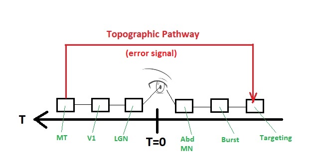
Two things of note are first that a targeting command from MT equates with the artificial introduction of an error signal, and second that MT has to know what parts of the incoming visual information pertain to the targeting command that happened 7 ticks ago. This means MT has to keep its output around for a while. Call it... working memory. Even in this simple system, things can get complicated pretty fast. There are three inherent behaviors that must be fulfilled: fixation, tracking, and saccades (including their respective reflexes). At this level though, all we have to do is self-organize the integrator so it correctly tallies the incoming bursts and holds the designated eye position. This is just setting the gain. The gain is allowed to self-organize "such that" the amplitude of the muscle contraction exactly corresponds to the target position, and this is just a negative feedback loop. The translation from retinal coordinates to muscle coordinates is handled by the targeting system and the burst neurons.
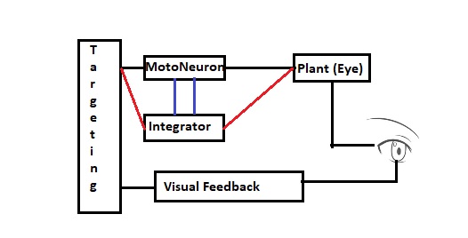
The figure shows multiple possible arrangements for the integrator, in red and in blue. The biological wiring supports both mechanisms. Which ones should we use and in what combination? This is another area where modeling can help us. Careful analysis of human eye movements reveals at least a part of the integrator action, and we can infer much of the rest from results with non-human primates. In a real human, the horizontal integrator lives in the nucleus prepositus hypoglossi (NPH), which works in conjunction with the medial vestibular nucleus (MVN). There is a separate integrator for vertical eye movements, in the interstitial nucleus of Cajal (INC). These systems develop after birth, in the first few weeks after the intial exposure to light. Since the targeting system in the superior colliculus is retinotopic, the eye movement has to be separated into its principal axial components. The two well known ways of doing this are with dot products and cosine angles (which turn out to be the same thing in Euclidean geometries), and neural networks are especially adept at calculating dot products (as they are just multiplications of the input vector by the weight matrix). What remains then, is a way of translating the geographic coordinate to a burst amount. The idea is, the farther away the target is from the fovea, the bigger the motoneuron output will be, because a bigger muscle contraction (eye movement) is needed to foveate an eccentric target. Thus from the targeting system to the motoneurons, we can have a gradient of connectivity, with the most eccentric targets causing the largest muscle contraction and thus having the greatest connectivity.
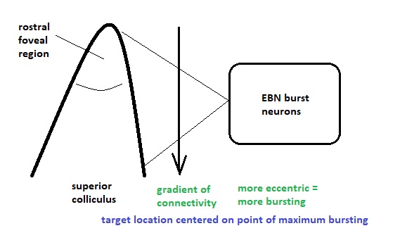
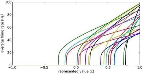
Such gradients are ubiquitous in biology. They're all over the human brain, including both peripheral and central areas. The population of motoneurons must calculate and represent an "amount" of muscle contraction, which is just a single value. Thus we wish to know whether encoding mechanisms are at work, for example we'd like to look at the variability of the current-frequency curves in the population of motoneurons. This graph was shown earlier in relation to the Seung model. It clearly shows that there is a large variability in these curves, making it very likely that the population of abducens motoneurons is encoding a value that arrives in the form of "amount of stimulation" from the topographical gradient in the targeting system. Between the targeting system and the motoneurons, are the burst neurons and the integrator. So we now have to consider the control system at a finer level of resolution.
In humans, the timing around the oculomotor loop is pretty tight. EBN activity begins 11-12 msec before a saccade, which is just enough time for two synapses (presumably these would be the one from the EBN to the abducens motor neuron, and the one from the motor neuron to the lateral rectus muscle). However there's still an issue with the control loop. To derive an appropriate error signal, we need the amount of mismatch between the target and the fovea. How do we get that? On the retina is an image consisting of many possible targets, including the one we want. How is the desired target separated from all the rest?
Ultimately this question can only be answered by the visual system. First the object needs to be given a bounding box, then the center of mass needs to be identified, then the coordinates of interest relative to the center of mass can be specified, and so on. Part of this information is used to select the target, but once the target is selected, another part of the object-related information is used to focus precisely within the target area. Sometimes it doesn't matter exactly where the active focus begins, but sometimes it does. This places stringent requirements on the targeting system, since it's not necessarily true that peripheral targets are less important.
Once having a unique set of target coordinates though, we still have the issue of translating those into muscle contractions. The projection onto coordinate axes is straightforward, however these axes are only needed at and below the level of the EBN burst neurons. There are schemes that allow the simultaneous calculation of dot product and target vector, as long as a closed loop control output from the oculomotor muscles is not needed. This latter issue is somewhat thorny insofar as it involves the palisade endings, which are still controversial, however ultimately in humans there is no behavioral need to move the eyes to a specific angle in the absence of a visual stimulus, and in fact many people find that learning this behavior is quite difficult. The control loop seems to be closed by the visual image itself, which drives both saccades and pursuit movements.
Therefore we can have an open loop ballistic phase at the beginning of a saccade (which dovetails with human physiology), until such time as the visual control loop can activate. One of the closed loop's most important functions is turning off the saccade, which should be done precisely on target, and therefore the loop should be predictive of the target location at the time it's turned off. Mapping this onto the timeline, we can thus clearly see the need for several types of control loops, and in a real brain the existence and timing of these loops can be verified with white noise analysis. For immediate purposes we'll use a simulator to find out which integrator arrangement gives us the best (most biologically consistent) results.

The dependence on a gradient for converting a spatial map to a value is an ubiquitous motif in neural networks. Such a mapping can occur with or without current-frequency encoding by the postsynaptic population. With such encoding, the learning process is straightforward and very fast. Without it, learning can be slower but also more linear. The idea of a homogeneous population of neurons separated only by variability is different from a spatial topography, because a clump of neurons is not even one-dimensional, it's just a point. It's effectively 0-dimensional.
The model results are shown using the Nengo simulator. In this case the number of abducens motoneurons has been reduced from 6000 to 60, in favor of computation time. This number is adequate to represent a single value. The population of abducens motoneurons has been designated an Ensemble, as has the integrator. The integrator is constructed with positive (excitatory) recurrent synaptic feedback. The neuron properties are distributed randomly, and the synapses are programmed to learn the gain that makes the eye position equal the target position, based on a visual error signal.
(figure from Nengo)
Now let us consider two different kinds of self organization that occur at a higher level. First, there is the topographic organization of the optic radiation and its modular organization at the level of the cerebral cortex. Then, there is the mapping between the cerebral cortex and the oculomotor targeting system in the superior colliculus. Much is known about the former, and less about the latter. To explore topographic mapping, we first need the concept of a neighborhood, and then we can define the convergence and divergence of neural connectivity.
Topographic NetworksAt this juncture in the discussion, topographic networks have been loosely equated with CNN's (convolutional neural networks), at least in the context of the retinotopic visual system. In this analogy the convolutional kernel is related to the convergence and divergence of the neural connections, and could in many cases be considered hard-wired. This is not the case in real brains, as shown in the section on the retina, where even in the most peripheral nervous system, the receptive fields are modulated and controlled by both environmental input and central processes. And artificial CNN's do not generally engage in lateral inhibition, instead they attempt to incorporate this effect statically at the level of the convolution kernel. The result is that the kernel never changes, as distinct from a receptive field that's constantly changing.
In a digital monitor, each pixel has a coordinate and an RGB value (a word). The coordinate is usually defined by a location in memory (it is "geometric"), which contains the associated data. Computer memory is 1-dimensional, so the pixel arrangement in memory is automatically vectorized before it reaches the neural network. The colors can be separated by masking off the unwanted portions of the data in memory. In contrast, in the human visual system, each "pixel" has attached to it four colors, on and off times, velocities, spatial and temporal frequency information and dynamics, and possibly systemic information related to ongoing oscillations. Instead of three values per pixel, the retina outputs several dozen. These are then further integrated in different ways in the LGN. Each of the six layers leaving the LGN (plus the koniocellular strands between the layers) contains multiple channels (on cells, off cells, etc) which then multiplex into various layers in the cerebral cortex. All of these pathways are topographically specific.
In the primary visual cortex there are 140 million neurons on each side, compared to just 1 million leaving the retina and 6 million in the LGN. The topography of the cortex is such that each mini-column consisting of about 60-80 neurons corresponds with approximately one point on the retina, and thus we expect a complete set of orientation columns and ocular dominance columns with their accompanying blob to cover a retinal territory equivalent to about 80 photoreceptors. This is approximately correct given what we know about the connections between photoreceptors and bipolar cells, bipolar cells and retinal ganglion cells, and ganglion cells and LGN relay neurons.
(figure)
To calculate the mapping target of a projection, one first determines the corresponding geometric location in the target topography, then one applies a divergence which is an "extent" of connectivity, possibly having a shape. The divergence is frequently related to axon and dendrite branching, and sometimes it can be directly calculated based on branching shapes (including tree-like fractal branching patterns as well as lateral connectivity inside neuropils). A k-nearest-neighbors algorithm is frequently used, where k is the divergence.
(figure)
The salient feature of a topographic map is that its coordinate system is maintained through the mapping. In general there will be both neural gradients and macroscopic brain topography overlaid on top of the connection map, however the underlying coordinate transformation can always be described by the synaptic weight matrix Wi,j. If the input to a layer is X(t) and the output is Y(t), then
Y(t) = f ( Σ Wi,j(t) * X(t) )
where f is a nonlinear threshold function (usually sigmoidal, logistic, ReLU, etc), and unused or non-existent connections are assigned a weight of 0. In a 1:1 point-to-point topography Wi,j = 0 for all i != j, whereas in an omniconnected topography we must sum over all inputs. In a convolutional architecture the kernel usually covers some combination k of nearest neighbors, so we might have a function like [ d(Y,X) < k ] multiplied by a weighting factor based on the distance d. In all cases, the maps X and Y must be aligned in order to calculate d. If we have source and destination manifolds we must convert to a common coordinate system first, do the math, and convert back. Since these networks mainly work on correlation, it is important that we be able to map and parametrize non-Euclidean distributions. This topic is treated by information geometry, which we'll consider after we look at some modeling tools.
Speaking of modeling tools, there is an important gap in the landscape when it comes to geometry and topography. It is extraordinary difficult in most cases to assign complex topography to a layer of neurons. With the current state of the art, it would be nearly impossible to accurately represent even a very small patch of visual cortex, because the geometric layout tools are simply not available. There are many approaches that hover all around the target, but never quite hit the mark. Allen Institute has some lovely brain maps but they haven't done anything with meshes so can't accurately represent the boundaries of any of the internal structures. Neuron simulators abound but none of them do anything with topography except in the most rudimentary (and generally useless) manner. Geometry tools exist, but they're mostly in the computer graphics and animation space, and scientists don't necessarily want to deal with vertices and polygon faces when they're trying to model the connectivity of a curved brain structure. Today, it's sometimes easier to roll one's own and quickly program a small scale simulation using NumPy. This is the approach taken in the section below. It is adequate, it tells the story.
Self Organizing MapsIn self organizing maps, it's the coordinate system that changes, not the underlying data. A self-organizing map will find the coordinate topography that best describes the data.
Self organizing maps can work on competition and cooperation, and they can also work on correlation. Imagine there is a retina R, and a visual cortex C. The nerve fibers from R have to find their targets in C, and the topography has to be maintained in the mapping. This will be a two dimensional mapping, in retinal coordinates, and we'd like to be able to use Cartesian coordinates or polar coordinates, whichever happens to be more convenient at the time. We'd like the topography to self-organize, and we'd also like the synaptic strengths to self-organize. (Sometimes we get lucky and those are the same thing, but sometimes they have to be separated).
We can approach this scenario from two different directions simultaneously. The first is, we can stipulate that each map (source and destination) has a pair of marker molecules whose gradients "approximately" determine the position of each neuron. And second, we can specify the learning rule, and the mechanism by which changes in synaptic strength occur. With this network architecture, a competition-cooperation calculation is often considerably faster than gradient descent.
Before we look at connecting two coordinate systems, let's look at what happens within a single coordinate system. Let's imagine we have a neural network layer we'll call C, and it initially has some kind of regular arrangement (specified by its pair of marker molecules, which together form a coordinate system). And we'll feed another layer into it, we'll call the input layer R. R will also have a coordinate system specified by two marker molecules, but initially for this first demonstration we won't align anything, we'll just say there is "some mapping" between source and destination. The connection from R to C begins with axons elongating in the direction of marker molecules. Once they find their targets (where there is the greatest concentration of markers), they begin to sprout, connecting with postsynaptic neurons. At first they branch widely, connecting with many targets, but gradually once data begins to flow the eccentric connections are pruned away and what's left is a very regular connection geometry. In humans such a topographic connection process can take anywhere from a few weeks to 200 or more days. The first part is always axon growth in favor of connectivity, and the second part is always synaptic pruning in favor of the topography.

To set up the initial synaptic weights, we can take a random distribution with a small positive mean and a small variance. Now we will begin to stimulate R in three specific locations, as shown in the animated figure above. What we notice is that the synaptic connections are strengthened in such a way that all the weights move towards the stimulation sites, they cluster around the places where the input is. The particular learning rule in play is determined by the biochemical mechanisms underlying the synaptic transmission in the network. In many cases the synaptic transmission is complex, involving more than one neurotransmitter. Sometimes the complexity only occurs after initial network organization, but sometimes it's an essential part of the organization.
Correlation MapsIn the correlative version of self-organization, the network is responding to the simultaneous occurrence of signals at two different points in space, which in this case corresponds to the statistics of the input. During training, we never show the network random dot stereograms, we always show it real objects - things with edges, contours, and surfaces. If we were to show it random (white) noise instead, there would be no correlations among the inputs, and therefore the synaptic weights would fail to differentiate.
It's a very short step from a self organizing map to an associative memory (Kohonen 1989). We can extend the mapping paradigm to the case of an associative memory, by simply splitting the input into two parts. If we have X(a) and X(b), and there is no autocorrelation, then the network will come to respond to the correlation between a and b. If there is auto-correlation, even within a single image, then the autocorrelation will be represented in the network. In this way, a self-organizing map based on correlation will find the coordinate system that best matches the organization of the input statistics. In the language of statistics, we say that the network learns the distribution of the input. For this to happen, it is important that the representation of the image in the network "approximately match" the real statistics, in other words if the network is processing the distance between edges, then that distance should fall within the boundaries characteristically displayed by the data. In a human environment walls can typically be at opposite edges of the visual field, whereas the legs of a fly are very close together, therefore the visual system must handle a broad range of spatial frequencies. On the other hand there are rarely abrupt discontinuities in the time domain, unless they are due to occlusions or other interactions between objects.
In a recurrent associative memory, separable data is individuated by the placement of suitable attractors in the phase space. Showing such a network a portion of an image that has already been memorized, will start the network near the attractor, and in a few short ticks the network will locate the attractor as a local energy minimum. When two images are associated with each other, the representations tend to cluster near each other in the phase space, thus presentation of one image will locate the attractor and emit either the other image, or oscillate between the two coupled images.
Buffer MemoryThere is one type of self-organization that requires movements to be precisely timed, and there is another type that doesn't care much about timing and instead extracts invariances. Are these the same? Is there a common underlying mechanism? The good news is that yes, there probably is. The bad news is that it uses a library of dozens of different kinds of plasticity. Each variety is good for something specific, and the brain uses whichever one is best suited to the task at hand.
Visual scene reconstruction requires a buffer memory to hold previous scenes belonging to the same episode. This is useful for both contextual recall and episodic storage. One of the interesting aspects of associative memory is how to recall a "subspace" without recalling the whole information field. For example if there are two clusters in memory, one called "table" and another called "chair", and we are shown an image of a chair, we'd like to be able to recall the relevant subspace without having it cluttered by irrelevant information about tables. This means our associative memory should have some advanced dynamic properties, and it also means that there should be a temporary memory that can hold one or more subspaces as long as they're in active use.
The most important realization though, is that such a memory requires a control system. A dynamic memory in a computer might require an occasional refresh, and the cache contents might be replaced fairly regularly depending on the activity of the user. The brain is no different. When someone is navigating a scene, and is then interrupted and asked to navigate a different scene, the information about the new scene must be loaded into memory. This takes time, and the time it takes can be measured, under the appropriate experimental conditions.
Considering this in terms of a short-term buffer (which is essentially a cache), the contents of such a memory will be determined directly by the synaptic weights in the network, and thus the process of loading the buffer involves programming the synaptic weights (and similary, clearing the buffer involves resetting the weights). Such activities might occur for example, in relation to a P300, as well as in the normal course of successive episodes. Programming a set of synaptic weights is a perfect reason for neuro-modulation. Modulations occurring via metabotropic receptors linked to second messengers are known to be able to affect receptor kinetics over the longer term. Such mechanisms have been found in the hippocampus, cerebellum, cerebral cortex, and elsewhere.
Next: Data-Driven Organization |