To model the visual and oculomotor timeline, we'll build a little self-organizing robot with two eyes that move. The visual part is to be able to identify potential targets ("objects") in the visual field, and the oculomotor part is to be able to foveate and track a selected target. Once these parts are connected, we will have all the basic varieties of human eye movements in place, including reflexes. Along the way, we'll have to build up a rudimentary vestibular system so we can support the VOR.

When we have a functioning timeline, we would then like to be able to move the eyes between targets. We will thus raise a prototype "attention" system, that prioritizes targets in a number of ways. To support an attention function, we'll need visual memory too. If this sounds ambitious, don't worry - it's not that hard! Our goal is to get close to an autonomous exploratory behavior, and for that we'll need more than just an eye movement system, but we'll get to it when we get to it. Let's decide on the overall architecture of the model, then we'll do the visual part, and the oculomotor part. Once those are in place we can see if we can connect them together.

You may ask why we would want to do this. The short answer is, we want to test the Timeline Model. We'd like to see if it brings anything new to the table, that ordinary descriptions of time-locked neural activity have difficulty with, or otherwise don't account for. A theoretical understanding is one thing, but when we try to actually build something, all the little details and nuances become important, and generally after an engineering effort we end up understanding the science a lot better too. In the famous words of Richard Feynman, "I don't understand anything I can't build". (Feynman has a lot of great quotes, like "I would rather have questions that can't be answered than answersthat can't be questioned", and "scientists are explorers, philosophers are tourists". (grin :)

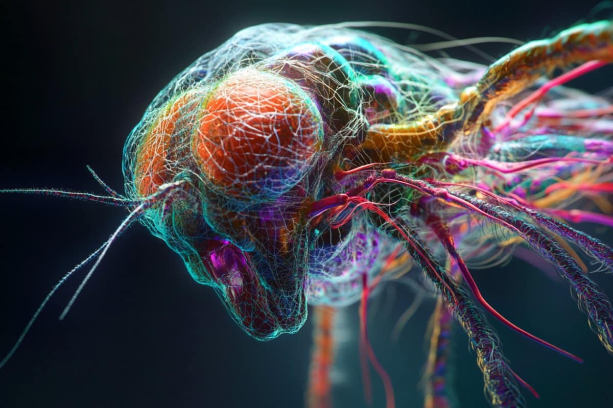
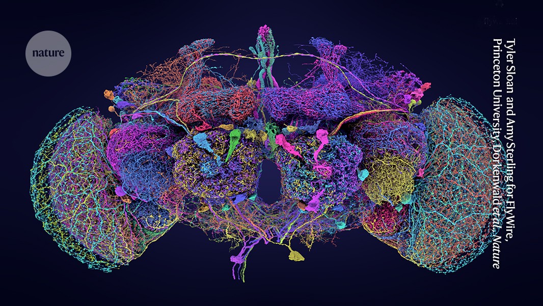
We should mention at this point, that the approach of a self-organizing robot has already been tried, with very good results, on the fruit fly Drosophila (Goldsmith et al 2024, Lappalainen et al 2024, Iwasaki et al 2025). Recently researchers at Princeton University mapped the entire brain of Drosophila down to the synaptic level (NIH 2024, Schlegel et al 2024, Dorkenwald et al 2024), an amazing accomplishment that couldn't have been completed (in our lifetimes) without the help of AI. FlyBase is an excellent resource if you're interested.

Just because the pictures are so cool, here is a fruit fly. Can you imagine making a robot out of this? Wow.

And here is the brain that controls a real fruit fly (it has about 140,000 neurons):

The Linear Timeline

Our first task is to build the network geometry. Since this is a real time model, the first thing we'd like to do is construct a linear mapping timeline, based on what we know about the neural structures in the visual and oculomotor systems. How do we do that?

The first step, is to take a careful look at the network architecture. What's the first thing you see, when you look at the visual system? Topography! Lots of point-to-point geometry. So we'll definitely need a tool that can handle that for us, and moreover it has to be quick and interactive, because we're going to need to change the geometry repeatedly, to investigate its relationship with network behaviors. For example, the LGN is a curved structure. Does it matter? Do we lose anything by modeling it as a flat sheet of neurons?

Next, we have some basic connection motifs in our brains, that repeat over and over again in different systems and contexts. Lateral inhibition, is one such motif. Feed-forward inhibition is another. We need our geometry tool to handle lateral and recurrent interactions as well as the feed-forward connectome.

And, as we begin this modeling effort, we don't yet know everything that will be required of us in terms of neurons. In ANN's as with all engineering, there's always more than one way to do something. It depends what the goal is. If the goal is biological realism then we need to model things like retinal adaptation and the dynamics of receptive fields. On the other hand, if we just want to see information flowing through our network we could use an unbiological tool like TensorFlow, which is very good with feed-forward geometry but has difficulty with lateral connectivity.

A real human retina has 100 million rod photoreceptors, but we don't need that many. For modeling purposes, we can live with a small patch of retina to begin with, let's say, 10,000 neurons. That may seem like a lot, but it's not really, because in a two dimensional sheet it's only 100 neurons on a side. Which is probably not enough, but it's a good start. Let's see if we can lay out a 100x100 patch of retina. From the machine learning point of view we basically have flat sheets of neurons that connect to each other in interesting ways. We know the feed-forward paths, like receptors => bipolar cells => ganglion cells, and to get the lateral paths we just have to look inside the neuropils. Let's begin with the simple approach and do what the machine learning people do, which is focus on the forward path. How can we build this?

Sadly enough, none of the popular neural network modeling tools can handle this for us, at least not in a user friendly way. There used to be a tool called Topographica that came close, but it's no longer being supported. (If you're a computer expert, it would be a great project to bring this into the 21st century with Python 3 and all the updated libraries).

Without the topographic modeling capability we're in trouble right from the beginning. There are all kinds of ways to kloodge around the issue, but at the end of the day the biological connection motifs need to be supported, because otherwise we're doing machine learning and not neural network modeling. So let's take a look at one way this will work. This is a simulation "interface engine" that I wrote myself, it's called Annie. It stands for "Artificial Neural Network Interface Engine". It takes a simple definition file as input, and outputs a complex data structure that completely describes the network, down to the synaptic level. The code is available for free on GitHub, it's written in Python and will run on any operating system (even in a cell phone, with an app called Termux).

First let's look at how we can do geometry (the retina being an important and simple example), and then we'll look at how to apply what we've learned to the timeline.

The Annie Interface Engine

Annie takes a simple interface definition file as input. We'll use the retina to illustrate. A human retina seems pretty simple, but it's actually very complicated. There are 40+ different kinds of amacrine cells, and 20+ types of ganglion cells, that have been identified both genetically and anatomically. But the basic structure is pretty straightforward, there's basically three feed-forward and two lateral layers with two neuropils called the inner and outer plexiform layers. The weirdness in the geometry is that there's a blind spot where the ganglion cell fibers exit to the optic nerve, and the distributions of the various cell types differ with eccentricity.

Before beginning, we need to define a coordinate system. Euclidean seems best at this early stage, later we can consider whether other geometries might help us, but for now we can go with the Euclidean 3-d, because that will also allow us to interface with graphics and animation software, which we'll see in a moment is entirely necessary. So we'll just pick some coordinates, say, 10,000 units along each axis. We'll create a definition file called "retina.in" that begins like this:

NETWORK RETINA
      COORDS (10000,10000,10000)

This defines our coordinate space. Now we need to insert sheets of neurons into this space. But wait... there's already something missing! How do we stimulate our photoreceptors? We'll need some light. And, we'll want to run experiments with this retina, the same way the scientists do - we'll want to present flashes of light, moving points of light, annuli, bars, and gratings. So we'll create a second file called a Stimulus Template that defines how the light behaves. It looks like this:

TEMPLATE BARS_1.IN SIZE (300,300,0)
      BAR (0,0,0) TO (100,100,0) LEVEL 5.0
      BAR (200,300,0) TO (300,300,0) LEVEL 5.0

Fine, done, we have two bars of light, so save the file and return to the retina. After defining the global coordinate system, we need to insert our sheets of neurons. We can do it this way:

NUCLEUS RETINA
      CENTER (9000,9000,9000)
      EXTENT (800,800,800)
            CELL RODS
                  CENTER (9000,9000,8800)
                  EXTENT (500,500,5)
                  NEURON_SIZE (5,5,2) VARIANCE (2,2,1)
                  NEURONS 10000
                  ARRANGEMENT GRID_2
                  NEURON_TYPE LINEAR

In this example we've told the interface engine to lay out 10,000 neurons in a two-dimensional grid. Now... this is a little painful, if we have to do this for 20+ ganglion cell types our definition file can get a bit long. A different way to do this would be to have an interactive GUI tool that lets us lay out networks. Such tools did and do exist, the problem in the past has been that the computational part attached to the neurons has been sub-standard and inconvenient. And we should also mention, that this approach of a network definition file is used in other simulators, like Nest. XML is definitely painful though, the simple approach embodied in Annie is much easier and more user-friendly. (Annie will export XML, if you need to interface to Nest).

After defining all the cell types we want, we have to define the connections. And this is where the geometry starts making demands. There are two "neuropils" in the human retina, the inner and outer plexiform layers. Axons enter these layers and branch laterally, making synapses with the dendrites of other neurons which also enter the layer. So before we define the connections we have to define the neuropils, like this:

NEUROPIL OUTER_PLEXIFORM_LAYER
      CENTER (9000,9000,9250)
      EXTENT (500,500,5)
      USED_BY BIPOLAR_CELLS
      USED_BY AMACRINE_CELLS
      USED_BY GANGLION_CELLS

As before, we just give the neuropil some geometry, and now we can insert connections into it.

CONNECTION FROM ON_BIPOLAR_CELLS TO AMACRINE_CELLS
      TYPE AXODENDRITIC
      DIVERGENCE 5 VARIANCE 2
      WEIGHT 0.2 VARIANCE 0.05
      TOPOGRAPHY POINT
      USES OUTER_PLEXIFORM_LAYER
CONNECTION FROM AMACRINE_CELLS TO AMACRINE_CELLS
      TYPE LATERAL
      TYPE DENDRODENDRITIC
      TYPE BIDIRECTIONAL
      TYPE INHIBITORY
      DIVERGENCE 4
      WEIGHT 0.1
      USES OUTER_PLEXIFORM_LAYER
CONNECTION FROM ON_BIPOLAR_CELLS TO GANGLION_CELLS
      TYPE AXODENDRITIC
      WEIGHT 0.25
      TOPOGRAPHY POINT
      USES OUTER_PLEXIFORM_LAYER
CONNECTION FROM AMACRINE_CELLS TO GANGLION_CELLS
      TYPE AXODENDRITIC
      TYPE INHIBITORY
      WEIGHT 0.2
      USES OUTER_PLEXIFORM_LAYER

... and etc.

In this example, we've defined the feed-forward and lateral paths through the outer plexiform layer. What will happen is every neuron type has been specified as a 100x100 sheet and thus will be laid out in a well defined grid, according to the specified coordinates. The connection between amacrine cells has been defined as DIVERGENCE=4, therefore each cell will connect with its nearest neighbors. The designated cell types will connect into the outer plexiform layer, but we haven't told Annie how to do that yet. This is how we do it:

CELL AMACRINE_CELLS
      CENTER (9000,9000,9600)
      ...
      AXON DIRECTIONAL (0,10,0) VELOCITY 1
            USES OUTER_PLEXIFORM_LAYER
            GEOMETRY DIPOLE
            WIDTH 5

Because the Axon has been specified as a dipole using the outer plexiform layer, and in the absence of further instructions, Annie will build the axon from the amacrine cell straight into the OPL, where it will branch in the specified direction with the specified width. There are many other geometries available, Annie is aware of apical and basal dendrites, tufts, and all manner of connectivity.

In addition to the retina itself, we will define two external nuclei, one called LIGHT, which is where our stimuli will come from, and another called OPTIC_NERVE, which is where our ganglion cell fibers will exit. These are two different examples of the usage of external nuclei, and there are many other examples too. In the first case we care about geometry, because when we do experiments, a spot of light has to be presented to a specific photoreceptor. In the second case we don't care about geometry (very much), as the virtual nucleus "OPTIC_NERVE" is just a collection point for axons to leave the retina. Now we'll take a look at the geometry we just created.

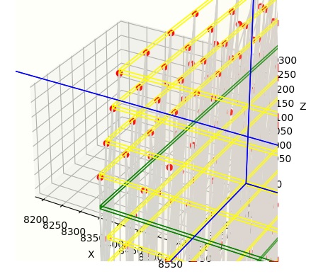
Upon completion of this exercise, the result is a retina, and two external nuclei. We have light coming in, and we have ganglion cell fibers leaving. Here is a graphical representation of what we just created:

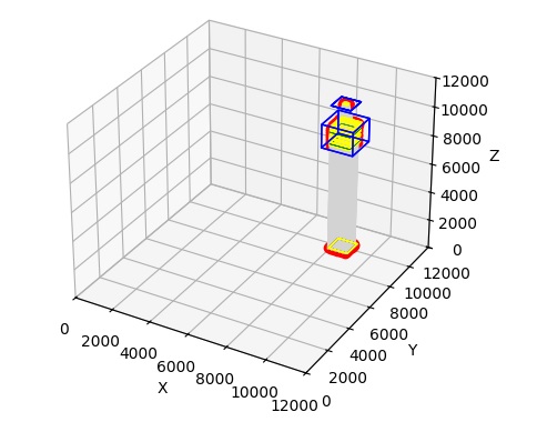
In this figure, light is at the bottom, and the optic nerve is at the top. You can see the stream of light entering the retina, that's the gray part. We can zoom in on the retina to see what it actually looks like.

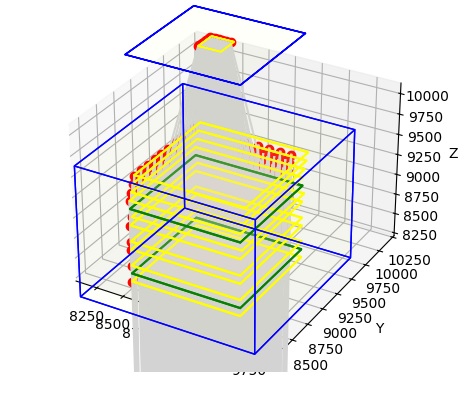
Now we can see the sheets of neurons, in yellow, and the neuropils, in green. And, we can even see a few neurons, in red. Also, we can see the ganglion cell fibers exiting the retina on top, collecting through a small piece of our OPTIC_NERVE. We can even zoom in farther, so we can see the individual neurons. In the figure below, the neurons are in red and the connections are in grey.

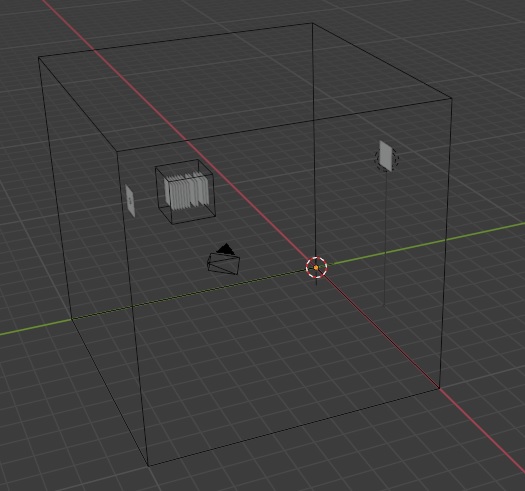
Python's matplotlib isn't the world's greatest presentation tool though (and we're trying to use it for something it wasn't really designed for), and besides, the retina is curved and all we have is flat sheets of neurons. What can we do with this? Well, one thing we can do is export this entire structure into a graphics program, like for instance Blender. Annie will generate OBJ files that are compatible with all of the popular graphics and animation programs, including Blender and Maya. OBJ files are defined in terms of "meshes", so in our case, each individual object we have defined will become a mesh, and its vertices and faces can be moved, transformed, shaped, and filtered to acquire whatever geometry we wish. Once we're done with the graphics engine, we simply export the results as an OBJ and read it back into Annie. Here for example, is the network we just created, in Blender. Note that Blender's Y and Z axes are reversed with respect to ours, so inside Blender, our vertical pedestal has acquired a horizontal orientation.

And here are our cell types, represented as meshes in Blender.

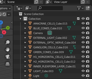
In the images above, there are no neurons and no synapses, because we are primarily interested in the geometric shape and arrangement of the nuclei, and the layers within each nucleus. What will happen is Annie will rearrange all the neurons on the way back in, when it re-reads the OBJ file exported from Blender. Annie will figure out how the geometry has changed and adjust everything accordingly. This is the trace from Annie:

export_obj(): 18 total objects
      144 vertices
      252 textures
      108 faces
import_obj(): imported 183 lines

Simple and elegant, yes? Sure... well... obviously, our simulation engine has to understand the network structure created by Annie. There are plenty of very excellent simulation engines available, so rather than try to re-invent the wheel, what Annie tries to do is export the network definition in a form that's compatible with the simulation engine of your choice. Mostly this involves defining neurons and synapses, because simulation engines rarely care which neuron belongs to which nucleus, they just dutifully transfer synapses into neurons and back into synapses again. (Although... there are many cases in which a simulation engine "should" care about geometry, for example when we're looking at anything having to do with astrocytes or volume conduction. However synaptic interaction is a good first target).

The Timeline Revisited

You can see, that in the retinal model we just created, we have the beginnings of a timeline. That is to say, we have sheets of neurons regularly arranged in a linear manner, with connections between them. In the retina though, each topographic location represents a point in the visual field - however in the timeline, each topographic point may represent an area of the brain, complete with all of its arriving and outgoing data. The timeline is, in effect, a retina that sees the whole brain instead of just a visual field.

Let's revisit our timeline. The timeline is a lot more complicated than a retina. A "sheet of neurons" along our timeline is a 3-dimensional volume of cells connected according to one or more motifs, and in the cerebral cortex these motifs becomes very complicated. A "processing mini-column" in the cerebral cortex consists of 100-ish neurons arranged in a very specific way, and a topographic "sheet" of such modules is multiply interconnected with its neighboring sheets. Trying to manage this architecture with definition files gets complex, but how else can it be done? Files are actually a very good solution, because they can be maintained in versions (on GitHub or with any popular source control system). And, files are very helpful to us when we want to run experiments. When it comes to the visual system, the idea of a set of "optical stimulus templates" we can re-use is stellar. Then all we have to do is tell the simulation engine which file to deploy at what time. An example could go like this:

SIMULATION RETINA_SIMULATION
      APPLY TEMPLATE annulus.tem TO LIGHT
            STARTING_COORDS (500,500,1000)
            MOVEMENT_COORDS (100,100,0)
            SCALE (100,100,0)
            START_TICK 2
            LOOP 9
            REPEAT FOREVER

When we're experimenting with our timeline, we'll want to present visual stimuli to the network, at the same time we're looking at eye movements. We'll definitely need the ability to start and stop our simulation on demand, and we need the results to be reproducible even in stochastic networks, because this helps us debug our network definition. Fortunately most operating systems have pseudo-random number generators that use a "seed", and if the seed is the same, the same set of random numbers will always be generated in the same order.

So now let's consider our timeline architecture again. At the far left of the timeline we place the hippocampal region, which will be our scene map and episodic memory. At the far right we place its counterpart the prefrontal cortex, which will provide mnemonic context for the scene map, and generate a distribution of possible motor behaviors for staging along the timeline. The point-to-point topography in the early visual system seems a natural for tools like TensorFlow, unfortunately it won't handle lateral inhibition for us, and therefore we have to move to something more amenable to biology. We have to find a simulator that will work for us.

In the next section we'll look at a very popular simulator called Nengo. One of the big advantages of Nengo (besides being by far and away the fastest simulation engine) is that the user interface is friendly and intuitive. Nengo understands Python code, it's a server than can support multiple simultaneous consumers. It also has a number of tailored back ends that can support everything from FPGA to neuromorphic chips like Intel's Loihi.