It seems we know quite a lot about the human visual system. Could we build a machine to do the same thing? Many have tried... the difficulty is that machines don't have dynamics (so far), and they don't have the genetic programming that codes for development of complex systems like the brain. Nevertheless, machine vision has seen a lot of success commercially, in things like facial recognition and the processing of high altitude images.

Human vision works quite differently from machine vision, but it's well worth studying machine vision in the areas where it's successful. One of the big differences between humans and machines is that humans are self-organizing. Our brains wire themselves, whereas a programmer or scientist needs to wire an artificial network. In the human retina for example, before the eyes even open, waves of electrical activity travel from the periphery to the center. These waves help organize the connections with and within the superior colliculus, and these connections end up aligned with the direction of "optic flow" as the organism traverses the environment. The retina knows on the basis of genetically programmed chemical markers, where the midline is along both horizontal and vertical axes - this is how it separates the visual fibers at the level of the optic chiasm, and also how the neurons map directional selectivity in both the retina and the superior colliculus.

Furthermore, the form and function of the many types of synaptic plasticity in the visual system are still largely unknown, and the internal function of the (visual) cerebral cortex is still mostly unknown. Machines that try to "see", are limited by the available technology, which today is great in the digital world and not so great in the analog world. However photonics is right around the corner, enabling dense computation with tiny amounts of energy, and the machine learning community is already creating layered systems with billions of simulated neurons.

In a real brain, the areas that we study, like the retina and LGN and visual cortex, are embedded into much larger systems. If we disconnect the other parts, the behavior changes. For example a simple lesion in the midbrain very close to the pontine visual and oculomotor areas can put a person to sleep, or even into a coma. The activity in the visual cortex is coordinated with other modalities in other areas of the cortex, by rhythmic electrical activity including alpha and theta waves, but also including high frequency components that were often filtered out in the early EEG research.

Another big difference between humans and machines is how we handle noise. Everything in biology is noisy and stochastic, very little is deterministic. Our neural networks take advantage of this noise, they make use of it - whereas engineers have been taught to get rid of it. A constantly changing input is vital for humans, our vision stops entirely if we don't have it. Our retinas adapt in seconds, and our eye movements fatigue after holding an eccentric position for 15 to 20 seconds.

How Machine Vision Works

Other than advances in camera technology, the biggest part of machine vision uses artificial neural networks. However these networks for the most part, are highly non-biological. In some cases the machines "emulate" humans, and in some cases they're specifically built to meet or surpass human capabilities. The machines tend to focus on visual data, because it's the only way they can be tested. Hence you'll see terms like recognition, classification, feature extraction, and pattern analysis used ubiquitously in the machine learning literature.

A machine vision network typically involves a long feed-forward path that eventually results in "recognition". An example is shown in the figure.

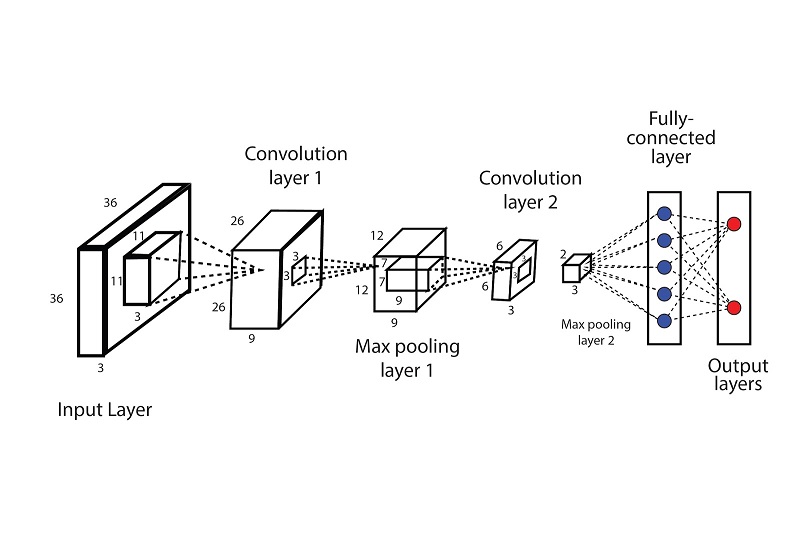
These are called "convolutional" neural networks. They are not new. They arose out of pioneering work by Kunihiko Fukushima in the 70's and 80's, in his capacity as a research scientist at NHK in Japan. Fukushima's "Neo-Cognitron" was the first translation-invariant convolutional network. His original network model is shown below.

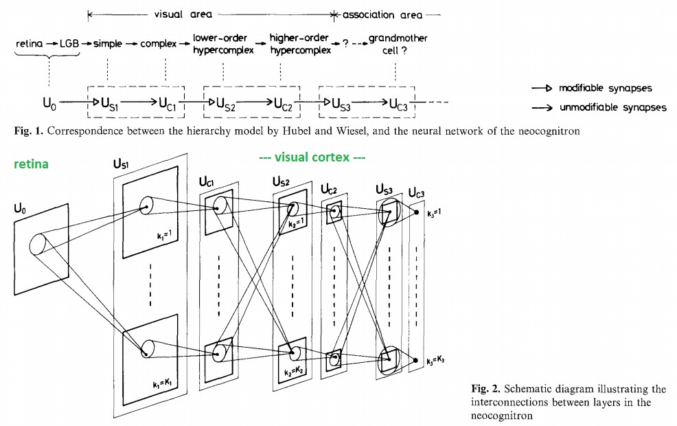
Note the parallel channels even at the level of the retina. Though the computational model is straightforward, you can clearly see that it was inspired by the brain. Modern improvements mainly revolve around processing speed and memory capacity.

The computations required of a convolutional network are well known, they closely resemble those occurring in animation software like Maya and Blender. A retina that sees an object in visual space is very much like a camera visualizing a perspective rendering.

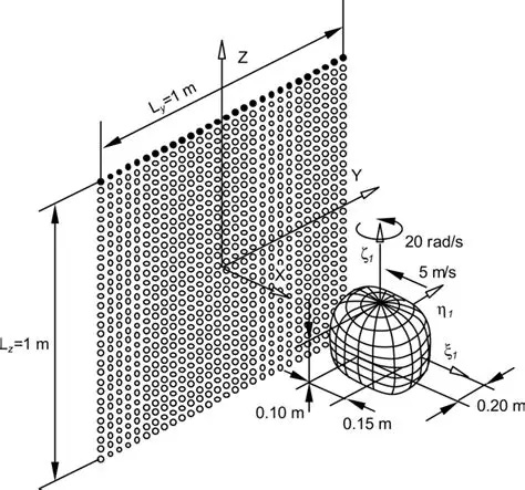
Downstream, from one convolutional layer to another, it is likely that information is being represented in the form of "manifolds", just like the object in the above diagram. Manifolds are surfaces, represented as correlations between nearby points. The representation of information in such networks is the subject of information geometry, which we'll look at in detail on subsequent pages. At some point it becomes important to understand the math. Early researchers into machine vision attempted to do everything geometrically, which rapidly became a nightmare, as the computer had to solve differential equations for every point in the visual space of both eyes. Later it became clear that much of the geometric information could be derived statistically, by treating visual images as point clouds and correlating the points. This kind of math replaces differential equations with a lot of matrix multiplication, and can often be made suitable for use with digital hardware like GPU's. The relationship between the geometric view and the statistical view is important to understand. In the early visual system in humans, the retinotopic mappings are determined by a guided competitive-cooperative processes during development, and then hard wired into place. This is a "massively parallel" architecture, maintained through at least the first few stages of the visual cortex. Instead of sweeping convolutional filters across an image like machines do, the human brain has an array of such filters that match the topography of the incoming visual signals. It can process in real time what the computers would take a long time to accomplish sequentially.

Convolutional Neural Networks

Artificial "convolutional" neural networks (CNN's) mimic an important aspect of human vision, which is spatial correlation, but they do it differently, in a way more suited to sequential digital processing rather than parallel analog processing. A digital convolution is like a small filter, that's swept across the visual field (or the "input space"). The filter looks a lot like a "Mexican hat" function, which looks a lot like the center-surround organization of a retinal ganglion cell. The filter is designed to emphasize contrast and de-emphasize noise. Convolutional networks are fundamentally patterned after biological systems. The requirements for human vision and machine vision are approximately the same. The mechanisms, however, differ substantially.

There are three main differences between the machine convolutions and the biological systems. First, in the machines the filter is swept sequentially across the image, which means the same filter can be re-used over and over again. However in biological systems the filters are hard-wired in the form of neurons and synapses, and everything occurs in parallel, so there is no need for nVidia GPU's to perform matrix multiplications - the calculations are performed by the network components themselves.

The second difference is that machines use feed forward architectures for computation, and back propagation for learning. A machine vision system is necessarily synchronized by a master clock, that first sends the information in the forward direction through the network, then sends the errors back the other way using back propagation. But there is no clock in the brain, and while there is synchronization in the visual system, it occurs in a different way. In humans, the pattern analysis portion of vision is interrupted by saccadic eye movements that occur about three times a second, and eye blinks that occur about once every three seconds. The brain uses this timing to coordinate sequential pattern recognition through rhythmic activity involving alpha waves in the visual cortex and theta waves in areas like the hippocampus and the claustrum.

The third major difference between humans and machines is that humans are noisy, and machines don't like noise. Humans are stochastic and noisy, every biological process depends on molecular interactions that have an imperfect probability of occurring, or occurring within an allotted time frame, or occurring unmolested. Relative to the statement that "machines don't like noise", there are exceptions. There are algorithms and components that have been built from the ground up using stochastic and statistical targets, and there are certainly algorithms that handle that aspect of the data better than others. In machine vision, more noise just means more computations. Whereas in biological systems, neurons wired in networks "use" the noise to accomplish more perfect correlations.

There are common elements too, between humans and machines. One of the things we learn from both humans and machines is that there's always more than one way to do something. The field of machine learning is only a few years old, it's still in its infancy. It started trying to mimic biological systems, and rapidly evolved along functional lines into things like large language models that have commercial value. Neuroscientists sometimes take an unrealistic view to what they're looking at, for example the matrix-like mapping of ocular dominance columns and orientation columns in the primary visual cortex turns out to be irregular and pinwheel-shaped, and this organization can be duplicated very precisely by a machine learning model that uses only the statistics of the data rather than any kind of inherent internal geometric organization. Both humans and machines are programmed by the data. Humans have meta-programming in the form of genetic instrutions, whereas machines rely on the cleverness of PyTorch and TensorFlow programmers.

Predictive Coding

So, how does all this information about neurons and synapses tie in with the timeline architecture and brain electrical potentials? Digital networks are non-biological and they don't have dynamics and they require 10,000 presentations of a face before they can recognize it (whereas you can do it with just one prior glance). Why are so many presentations needed? One of the issues is that the back-propagation of errors requires careful control over the learning rate because it works on "gradient descent". If the amount of descent is too little, the algorithm takes forever to complete. If the amount of descent is too much, the network starts oscillating wildly between random points on the energy surface, instead of descending gently to a minimum.

An alternative to back-propagation is predictive coding (here coding means in the neural sense, not like a computer program). The information ahead of T=0 on the timeline, is prediction, that's exactly what it is. An intended motor behavior can be staged along the timeline, but there's no guarantee that it will materialize at T=0. It may be inhibited before it ever gets there, or transmission can simply fail along the way. The common element of information along T > 0 is its predictive character.

Since its popularization in the insightful paper by (Rao and Ballard) the mechanisms around predictive coding have been extended by researchers like Karl Friston, who introduced the concepts of free energy and complexity into the basic paradigm. Free energy, in a neural network, is an indicator of surprisal. It has terms related to errors relative to previous predictions, and complexity related to the simplest possible description of the input.

The basic paradigm of predictive coding is easy to understand. There is an internal model that represents either the input, or the state of the network, or both. At time step t-1, the network will create a prediction of what it will see at t=0. It will then store the prediction. When the input arrives (or the network changes state) at t=0, it is compared with the stored prediction. The actual value is subtracted from the prediction to get an error signal. The error signal is then used to update the next prediction. (Communications engineers will recognize this as an adaptive Kalman filter, machine learning engineers might call it a Bayesian filter). The difference between this and a back propagation network is that errors are explicitly represented in a predictive coding network. They are encoded into the firing patterns of neurons. They are not "magically back-propagated between clock ticks", instead they are transmitted synaptically from one neuron to the next.

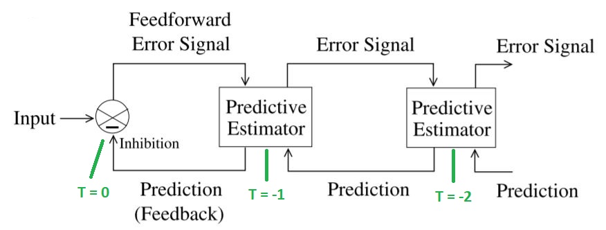
A simple neural network that accomplishes this is shown in the figure.

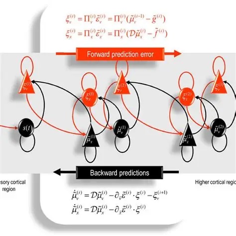
In a wonderful paper written from an evolutionary perspective, Pezzulo and colleagues describe how more complex architectures can be built up from this simple concept.

Over the last several years many variations of predictive coding networks have been created. There has been considerable focus on the various types of behaviors that can be supported by it. Unlike an RNN with back-propagation, a PCN can not be conveniently unrolled in time. However a PCN can provide significant performance advantages for moving images, especially when the motion information is pre-vectorized.

Stochastic Behavior

In college, engineers learn about control systems theory. First it's presented in a linear context, which always creates a few groans from the back row because it involves solving differential equations. But then the volume of groaning increases when the system becomes nonlinear, and the solutions become harder to find. The groans become an orchestra when students are asked to map dynamic behaviors into the phase plane - but then some magic happens, and everyone breathes a sigh of relief when it's discovered that complex systems can be approached statistically.

There is a difference between statistics and stochastic behavior. Statistics involves correlations, whereas stochastic behavior means noise. Correlative neural networks are driven by the data, which can be either noisy or not noisy. Stochastic networks are driven by the inherently noisy behavior of neurons, regardless of the composition of the data. The response of a neural network to noise depends on the character of the noise. In theory, white noise is uncorrelated with itself at any interval (noise is discussed in more detail in the section on modeling). Thus if the incoming noise is white noise, it will tend to cancel itself out over suitable intervals.

In a way, stochastic behavior is akin to the deliberate injection of noise. From a control system standpoint and the standpoint of the Kalman filters we discussed, noise is a way to overcome local minima, and the same thing applies to artificial neural networks. Stochastic behavior can be conceived in terms of random walks. The differential equations related to stabilizing a control system become stochastic differential equations, and can be solved using the methods of Wiener, Ito, Malliavin, and the like.

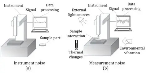
Conversely, a noisy system may exhibit process noise, and when we measure it we may also add measurement noise. These sources can be separated, and they can be removed from analysis but in many cases they affect the system dynamics and the trajectories in the phase plane. (A Kalman filter usually relies on a sensor for measurement, and humans rely on proprioception, both of which may exhibit measurement noise). In any control system we're interested in stability and convergence, and sometimes noise plays directly into the boundaries of stability. The figure shows an example of the difference between process noise and measurement noise. In this case the process noise arises from the instrument itself. In the case of a neural network, the instrument may be the preceding layer.

Machines can be quite good at extracting ground truth from noisy images. This behavior can certainly be accomplished by a simple Hopfield network, however in real brains we don't know the number of images or representations ahead of time. Large generative image networks have to be trained on millions of images, with varying shapes and placements, and the best approach for training seems to be to incrementally adjust weights and representations after each series of image presentations. Our brains probably use a similar method, both when they structure a scene from visual images, and when they consolidate only the essential information into long term memory. However it is still quite easy to fool an AI. Sometimes the alteration of a single pixel within an image is enough. A big part of the issue lies in what is being encoded. If pixels are being encoded directly, then pixels matter. If there is some pre-filtering between the pixels and the storage, maybe the individual pixels don't matter as much.

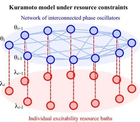
Dynamic Behavior

We looked at a simple example of dynamic behavior with the Wilson-Cowan network, and in a real brain this behavior becomes considerably more complex. One can build a robust, controllable, and adaptable oscillator from just a few neurons, perhaps the same number one might find in a cortical mini-column (say, about 100, maybe even less). When one has 100 million of these oscillators coupled together at different frequencies and phases, and they're all operating stochastically, even the Kuramoto approximation becomes inadequate to describe the resulting behaviors.

The Kuramoto model describes the behavior of coupled oscillators. In this diagram, each node could be an oscillator consisting of a small number of neurons connected into a simple oscillatory motif (for example in accordance with the Wilson-Cowan model). Coupling between nodes is accomplished by the (synaptic) connections between them.

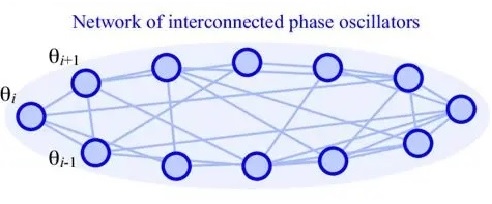
The basic Kuramoto model assumes that all the oscillators are at the same frequency. In real brains this is almost never the case, however there is "entrainment" of neighboring oscillators on the basis of the coupling between them. Depending on the coupling strength, different behaviors can be accomplished. One way of controlling the phase relationships is by adding an embedding network connected to each oscillator. With the proper network wiring, this embedding can effectively constrain the way each oscillator responds to the others.

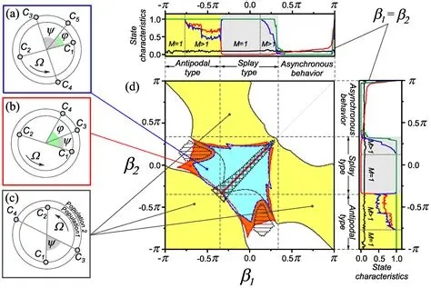
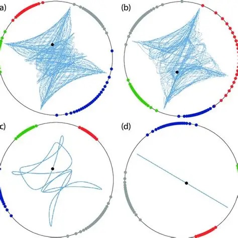
There are extensions of the Kuramoto model, for example the specific case of a bimodal frequency distribution has been solved exactly, for Lorentzian and Gaussian distributions. However the general case leads to a complex set of coupled differential equations that would be impossible to solve in real time with current technology. So we look for other avenues to approach questions like criticality, and one of the very promising avenues is nonlinear thermodynamics, which can be directly applied to neural networks with quantum computing. The complexity of Kuramoto dynamics is shown in the figures.

There is nothing like Kuramoto behavior in machine learning. Simply put, machines don't engage in dynamics. They depend on a clock, and that's it. Whereas, the fundamental method of system control in neural networks, is in fact the dynamics. The dynamics determine when a neuron will respond to its apical dendrites, and when it will ignore them. The dynamics determine the precise instant at which a neuron will generate an action potential. Trying to use spiking neurons without dynamics is non-sensical.

Learning and Training

Both machine vision and human vision involve three things: energy functions, error minimization, and synaptic plasticity. Energy functions are often called "cost" or "objective" functions. In machine learning paradigms, the cost functions are entirely arbitrary, they're determined by the needs of the programmer. Some popular and useful cost functions include those required for logistic regression, k-means neighbor analysis, and so on. In the thermodynamic (statistical mechanical) networks like Hopfield machines and Boltzmann machines, the energy function is defined by a Hamiltonian or Lagrangian, which is applied to the system dynamics and minimized. In free energy networks of the kind proposed by Friston, the cost function has terms related to information content and surprise.

We already looked at synaptic plasticity at a basic level, in the earlier section on synapses. Energy functions traditionally exist at the level of the network layer, although in non-layered systems like Hopfield networks and Boltzmann machines they may exist at the level of the whole network. In biological terms these might be equivalent to extracellular field potentials in some ways, and it is entirely plausible that these "neighborhoods" might have meaning globally as well as locally.

The term "error" is ubiquitous in machine learning, and it means many different things. Depending on the type of learning (supervised learning, unsupervised learning, and so on), "error" is measured against either a correct answer provided by the experimenter, or an internal model generated by the network itself.

There are also auto-associative networks that don't use "error" at all, instead they rely on spatial and temporal correlations to form relationships between features of the data. These networks were explored by Kohonen in the context of simple threshold neurons, and have been extended in many ways to include spiking networks. No model to my knowledge has yet explored the embedding of an auto-associative network into an electrical syncytium (of the kind formed by gap junctions in astrocytes). That would be a worthy PhD thesis, maybe even a career.

Kohonen's early models used competitive and cooperative interactions between neurons to model plasticity, instead of Hebbian learning. The difference is, that competition and cooperation requires interaction between multiple synapses, whereas the Hebbian model occurs locally within a single synapse. The first figure shows a Kohonen layer included into a larger network, and the second figure shows the feature-based clustering that's prototypical of a self-organizing map.

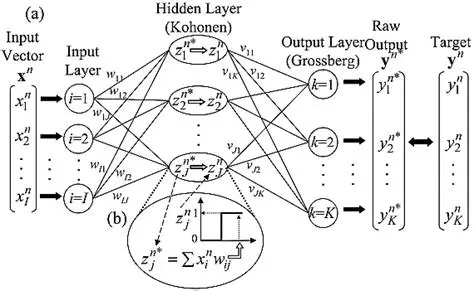
There is plenty of evidence for competitive and cooperative processes in biological systems, especially during development. When axons are first connecting to their targets, they "sprout", following by a period of "pruning". Much of the pruning activity depends on competition and cooperation between neighboring synapses, and the majority of it depends in turn on correlations and cross-correlations. Thus this type of map has a different purpose than data-driven Hebbian association, it's more related to topography and the wiring of neurons.

Let's take a closer look at the mechanisms underlying network plasticity, because there are many, and they all contribute to biological function. In the visual system, the plastic mechanisms are heavily engaged during development, and they don't simply "stop" during adulthood. For example, damage to the visual cortex generally results in the formation of new connections and the eventual recovery of function.

Essential Functionality

The essential functionality for both human and machine vision includes:

• Memorization
• Feature Extraction
• Classification
• Pattern Association
• Sequence Learning
• Attention
• Inference
• Generative Capability

Memorization

Two of the great strengths of the human network are our ability to store and retrieve memory patterns after just one exposure, and our ability to infer optimal sequences of action from sparse data. The basic ability to memorize can be accomplished in two ways: either alter the synapses to change the system trajectories, or alter the neurons themselves by programming specific spike patterns. The second method is biologically implausible, because human memory capacity greatly exceeds the number of neurons (it has been estimated at the equivalent of 2.5 petabytes of digital memory).

The easiest way to get a network to memorize an image is to simply burn it in. From a correlation standpoint, when the same image is presented again the result will be a 1, otherwise it will be a 0.

The machine learning community distinguishes between supervised and unsupervised learning, which is different vocabulary from the classical and operant conditioning in psychology. Unsupervised learning is akin to classical conditioning, where the repeated association of two stimuli leads to a mutual expectation. Supervised learning is more akin to operant conditioning, where there is a "reward" (or lack thereof) to indicate success or failure - in other words there is a "teacher" of sorts.

There are certainly many other forms of learning. One of the most important for humans is imitative learning, being able to repeat the movements of another simply by watching them. Apparently there are some specialized neurons in the brain that support this behavior, they go by names like "mirror neurons".

Feature Extraction

Once we are able to store an image so we can work on it, we'll be interested in extracting the high level features. For instance, chairs can be distinguished from tables on the basis that they have a back. When learning about chairs, we would like to give the network as many examples as possible, and each sample can be presented in several views. This way the network comes to learn the overall statistics of the feature set.

Image processing machines use many motifs commonly found in biological neural networks. For example the award-winning ResNet architecture creates "residual networks" consisting of feed forward connections that bypass layers. This architecture should be nothing new for neuroscientists, practically every set of connections in the brain has similar connectivity. However the machine learning people do the due diligence, they figure out exactly how bypassing contributes to better performance - whereas the neuroscientists tend to stop at the "look, it's possible" point.

Nevertheless, machine learning has not yet explored some important aspects of neuroscience. The so-called "residual connections" are ubiquitous in biological architectures, yet they were only introduced into machine learning about 8 years ago. Another unexplored area in machine learning is the multiple connectivity between two neurons, both from the standpoint of multiple neurotransmitters with different actions and time courses, and because there are sometimes a hundred or more synapses between any two biological neurons, and what is the purpose of these, when one synapse would suffice to carry the weight information? The obvious answer is "timing", and the machine learning community is just now getting up to speed on the meaning of timing within spike trains.

Recently neuroscientists have mapped the entire neural connectome of larval Drosophila (the common fruit fly), and as per the information transmitted in this outline, the entire network is organized on the basis of loops and there are very few unidirectional pathways. There are some interesting caveats to this general plan, for instance the learning part of the brain (Drosophila's associative memory) doesn't seem to have any loops, at least not in the larval stage.

Classification

A slightly more complex version of feature recognition is classification. You can show the network 100 pictures of cats and dogs and ask it to identify which ones are cats. We would like to obtain the category with the highest probability of fitting the data. For proper classification we need to look at the whole image, not just a subset of its features.

For example, the figure shows some people walking down the street, but there are also cars, dogs, strollers, and a variety of other visual information. What happens when we ask the network to identify all the "people" in the image?

Typically this question needs to be answered in stages, which is what the convolutions are for, in a CNN architecture. A person could be considered like a stick figure, two arms, two legs, a head, a torso... and people look different from dogs and cars. The separation of "people" from the rest of the image is a kind of classification problem, and we could even classify "within" the group of people, like show me all the men, or women.

Classification thus necessarily incorporates parts of the feature extraction paradigm. Successful classification occurs on the basis of the features in the image.

Pattern Association

Pattern association combines feature extraction with memorization. In the previous example we can extend the network's task by asking it to find all the men wearing NY Yankees hats. To do this, the network has to know that a hat goes on top of the head, and that dogs don't wear hats, and that we should ignore all the women wearing NY Yankees hats because we only want the men.

What are the combinations of features that will allows us to extract what we want? We need a surefire way of telling women apart from men. We could use long hair, but some men have long hair too (although a beard would certainly be a giveaway). We could also look for "fashion accessories" like purses (which men don't usually carry), and so on. In other words, it's the combination of features that will give us what we want. We are therefore correlating information within the image, instead of between images. If we want to do it between images, we have to memorize the images first, however if it occurs quickly enough we might be able to do it while the image still persists. Obviously, some short term memory might be helpful for us, so we can recall the previous views as they're needed.

Sequence Learning

Of course, in the real world, we do not simply receive static images from the machine learning engineer. Our visual field is dynamic, everything is constantly moving. The movie playing across the retina is no different from the audio in spoken speech, it is a stream of data that conveys meaning. Thus, we are interested in knowing the sequence of data, perhaps within a scene, perhaps across scenes, perhaps the properties a particular object across scenes.

The prototypical sequence learning machine is the RNN (recurrent neural network). This is a layer with self-recurrent connectivity, therefore in real life it can exhibit dynamics that include multistability and chaos. There are a number of ways of limiting the weight range in such systems, to avoid seizure-like activity.

From a computational standpoint, an RNN can be "unrolled" in time. This process is shown in the figure. This helps us computationally from a machine learning standpoint, because we can back-propagate derivatives all the way to the beginning of time. However it's also quite un-biological. We're just now beginning to discover how scene processing really works (with place and time maps in the hippocampus and so on), and it's already clear that there is substantial encoding before the information goes into memory, and at this point it's still entirely unclear how it's recalled. This is currently an area of intense research.

Attention

The word "apple" is ambiguous. It could mean a fruit, or it could mean a technology company. If I say "that apple was delicious", you can infer that I'm talking about a fruit. On the other hand if I say "my Apple broke", it's more likely that I'm talking about a computer. "Attention" in the machine learning sense, is a way of assigning context to data. As a heads-up, this usage is different from the way it's typically used in psychology.

A neural network derives context from memory (from "previous scenes"). If there is a word called "apple", the machine must execute a memory search for the context related to "apple". In the information that is returned, the memory subspace will have two distinct attractors, one for "fruit" and another for "technology company". To search memory, one must extract the search key from the image, and present it to the memory system "while" the image is still being processed. And, the memory search can not disrupt any other ongoing memory-related activities.

One of the things we've learned from machine learning, is it's very difficult to extract a subspace of the energy surface and use it to derive context. More likely, what happens is, an associative search through a Hopfield network will produce a sequential series of attractors, in other words the individual attractors will present in a sequence instead of all at once. The order they come out in, is related to their covariance with the search key, so there is no guarantee they'll come out in any particular order the way you want them.

Inference

One of the most powerful applications of artificial neural networks is in the area of inference. If there is a belief related to a model with some parameters, the neural network can fit the parameters to the data, "inferring" their values based on joint and conditional probability distributions.

A complete treatment of inference is beyond the scope of this short survey. However the landscape is pretty simple, the primary objective is to be able to navigate a graph with probabilites. The basic paradigm for machine learning is "Bayesian inference", where the posterior probability is updated based on incoming evidence. Fortunately the math around this is easy and straightforward. Bayes' Rule relates the posterior probability to the prior probability, as follows:

P ( Θ | X ) = P ( X | Θ ) * P ( Θ ) / P ( X )

where X is the input (the "evidence"), Θ is the model (containing the model parameters, which is what we're trying to find), and P is of course a probability. This equation reads: "the posterior probability is equal to the prior probability multiplied by the likelihood, normalized to the evidence". The likelihood is the term P ( X | Θ ), this gives the probability of the event before the new evidence.

Bayes' Rule is usually used to update belief in real time, for example if we have a time series X with points X_i arriving at times i=t, we usually recalculate the model at every time step i. However we don't have to do that, we can wait till the very end and use the "ensemble" of the input to make the adjustment. If we do this we may sometimes lose a little bit of data, so it's usually done once per input - but on the other hand, there is also a situation called "overfitting" where the network ends up thrashing around the answer, so in practice we have to balance performance against accuracy.

Generative Networks

Once we have the parameters of a model, we can generate examples from it. In the Bayesian paradigm, once we have decided on the model parameters Θ,
we can create examples from the model distribution. This can be done in a systematic way, to explore the organization of the memory, or it can be done randomly using a Monte Carlo approach.

The generation of examples from a distribution is not the same as adding "noise" to the input or the memory. If we have a model Θ, and we add noise to the parameters, we're actually changing the optimal configuration that was determined by our inference network. However if we get a sample first, and then add hoise, we're just creating a "noisy sample", and this can then be used to test the network's response to noise, and in associative memory experiments can be used to test auto-completion and overlap.
There is a special kind of generative network called "adversarial". This is a way of getting two networks to learn from each others' mistakes. In an adversarial network, there are basically two identical networks that feed each other models. The adversarial generator is creating "examples" from its own model distribution, and the other AI is looking at those trying to update its own internal model. This is a way of quickly exploring very large decision trees, for example the game of Go, or chess.